- Introduction
- Data
- Data Summary
- Exploratory Data Analysis
- Data Cleaning
- Data Visualisation
- Conclusions
- References
Introduction
I was inspired to analyse and visualise global fishing open data by the story produced by Jon Olav Eikenes.
This is also a sequel to my previous shark analysis post Is Swimming with Sharks Dangerous?, digging further into the potential reduction in shark numbers due to commercial fishing.
# Load packages
library(tidyverse)
library(sf)
library(rnaturalearth)
library(biscale)
library(cowplot)
Data
We will use the Global Fishing Watch Vessel Identity open data available with the Vessels metadata available under the Creative Commons Attribution-ShareAlike 4.0 International license.
Description: This table includes all mmsi that were matched to a vessel regsitry, were identified through manual review or web searchers, or were classified by the neural network. MMSI that are not included did not have enough activity during our time period (2012 to 2016) to be classified by the neural network (vessels had to have at least 500 positions over a six month period). If an mmsi matched to multiple vessels, that mmsi may be repeated in this table.
In order to download the data we need to register and sign into the Global Fishing Watch website. Therefore this data has been downloaded and saved offline.
First read in a sample using readxl package then read in the large csv file using the data.table package.
vessels_sample <- read_csv("vessels.csv",n_max = 30) ## Parsed with column specification:
## cols(
## mmsi = col_integer(),
## shipname = col_character(),
## callsign = col_character(),
## flag = col_character(),
## imo = col_character(),
## registry_geartype = col_character(),
## inferred_geartype = col_character(),
## inferred_geartype_score = col_character(),
## inferred_subgeartype = col_character(),
## inferred_subgeartype_score = col_character(),
## registry_length = col_integer(),
## inferred_length = col_double(),
## registry_tonnage = col_integer(),
## inferred_tonnage = col_double(),
## registry_engine_power = col_integer(),
## inferred_engine_power = col_double(),
## source = col_character()
## )vessels <- data.table::fread("vessels.csv",data.table = FALSE)Next retrieve the basemap data from the rnaturalearth R package. We will use the medium scale for zoomed out maps of countries. This dataset includes population and GDP values for 2016-2017.
# Get the world sf dataset from rnaturalearth package
world <- ne_countries(scale = "medium", returnclass = "sf")
# Check the class of world
class(world)
## [1] "sf" "data.frame"Data Summary
Let’s take a look at summary of the vessel dataset.
# View the vessels datasets
vessels_sample %>%
      glimpse()
## Observations: 30
## Variables: 17
## $ mmsi <int> 235050379, 412002468, 412068795, 41...
## $ shipname <chr> NA, NA, NA, NA, NA, NA, NA, NA, NA,...
## $ callsign <chr> NA, NA, NA, NA, NA, NA, NA, NA, NA,...
## $ flag <chr> "GBR", "CHN", "CHN", "CHN", "CHN", ...
## $ imo <chr> NA, NA, NA, NA, NA, NA, NA, NA, NA,...
## $ registry_geartype <chr> NA, "fishing", "fishing", "fishing"...
## $ inferred_geartype <chr> NA, NA, NA, NA, NA, NA, NA, NA, NA,...
## $ inferred_geartype_score <chr> NA, NA, NA, NA, NA, NA, NA, NA, NA,...
## $ inferred_subgeartype <chr> NA, NA, NA, NA, NA, NA, NA, NA, NA,...
## $ inferred_subgeartype_score <chr> NA, NA, NA, NA, NA, NA, NA, NA, NA,...
## $ registry_length <int> NA, 40, 30, NA, NA, NA, NA, NA, NA,...
## $ inferred_length <dbl> 24.30837, NA, NA, NA, NA, NA, NA, N...
## $ registry_tonnage <int> NA, NA, NA, 322, 362, 362, 470, 470...
## $ inferred_tonnage <dbl> 95.89842, NA, NA, NA, NA, NA, NA, N...
## $ registry_engine_power <int> NA, NA, NA, NA, NA, NA, NA, NA, NA,...
## $ inferred_engine_power <dbl> 344.6199, NA, NA, NA, NA, NA, NA, N...
## $ source <chr> NA, NA, NA, NA, NA, NA, NA, NA, NA,...From the metadata it appears that the flag refers to to the country codes.
flag: an iso3 value for the flag state of the vessel. Only for vessels that have been matched to registries or have known values.
# Reduce the variables to only required variables
vessels<- vessels %>%
      select(mmsi, flag, registry_geartype, inferred_geartype, registry_tonnage, inferred_tonnage)
View the vessels count by country.
# Count the vessels by countries
vessels %>%
      group_by(flag) %>%
      count() %>%
      arrange(desc(n))
## # A tibble: 232 x 2
## # Groups: flag [232]
## flag n
## <chr> <int>
## 1 CHN 137089
## 2 USA 25519
## 3 "" 17522
## 4 GBR 17009
## 5 NLD 16465
## 6 DEU 10645
## 7 PAN 9778
## 8 FRA 9316
## 9 NOR 8968
## 10 RUS 6292
## # ... with 222 more rowsThe countries with the largest number of vessels appear to be China, USA, Great Britain, Netherlands and Germany.
This table also shows the missing flags ie not matched to a vessel registry of the total 379693.
We will also take a look at the GDP figures by country. According to the Natural Earth release notes:
Admin-0 population and GDP values have also been updated to 2016/2017 vintage (primarily from CIA World Factbook).
Typically GDP is reported per capita (ppp).
world %>%
      select(admin,gdp_md_est) %>%
      st_geometry()
## Geometry set for 241 features
## geometry type: MULTIPOLYGON
## dimension: XY
## bbox: xmin: -180 ymin: -89.99893 xmax: 180 ymax: 83.59961
## epsg (SRID): 4326
## proj4string: +proj=longlat +datum=WGS84 +no_defs
## First 5 geometries:## MULTIPOLYGON (((-69.89912 12.452, -69.8957 12.4...## MULTIPOLYGON (((74.89131 37.23164, 74.84023 37....## MULTIPOLYGON (((14.19082 -5.875977, 14.39863 -5...## MULTIPOLYGON (((-63.00122 18.22178, -63.16001 1...## MULTIPOLYGON (((20.06396 42.54727, 20.10352 42....Data Cleaning
In the vessels data there are two variables, inferred and registry for each of the tonnage and the length of the vessels. We will assume that the actual values are with the registry values or the inferred if the registry is not available. The data quality is dependent on the data collection and neural network so we will also assume in this analysis that the data given is correct.
vessels <- vessels %>%
      mutate(geartype=ifelse(is.na(registry_geartype),inferred_geartype,registry_geartype)) %>%
      mutate(registry_tonnage=replace_na(registry_tonnage,0)) %>%
      mutate(inferred_tonnage=replace_na(inferred_tonnage,0)) %>%
      mutate(tonnage=registry_tonnage+inferred_tonnage) %>%
      select(mmsi,flag, geartype,tonnage)
Summarise the geartypes by count to view the categories.
# Count the vessels by countries
vessels %>%
      group_by(geartype) %>%
      count() %>%
      arrange(desc(n))
## # A tibble: 231 x 2
## # Groups: geartype [231]
## geartype n
## <chr> <int>
## 1 "" 236924
## 2 passenger 48239
## 3 cargo 18185
## 4 tug 11828
## 5 fishing 11640
## 6 tanker 10757
## 7 cargo_or_tanker 9953
## 8 trawlers 5547
## 9 non_fishing 4374
## 10 other_not_fishing 3994
## # ... with 221 more rowsThere are many different geartype categories. Let’s remove passenger, tankers and other non fishing vessels to focusing on fishing vessels. Since this is a large dataset this step also reduces our dataset size. This data cleaning is manually performed after visual inspection of the above data summaries so this is done on a best efforts basis.
# Remove vessels with no flag or geartype and passenger or cargo types to narrow down identifiable fishing vessels
vessels <- vessels %>%
      filter(!is.na(flag)) %>%
      filter(!is.na(geartype)) %>%
      filter(!geartype %in% c("passenger","cargo_or_tanker","other_not_fishing","non_fishing","gear","supply_vessel","tanker","cargo","research","","patrol_vessel","tug","dredge_non_fishing","cargo|passenger","seismic_vessel","non_fishing|trawlers","other_not_fishing|trawlers","bunker_or_tanker","reefer","bunker","cargo|passenger|supply_vessel","specialized_reefer","cargo_or_reefer","passenger|supply_vessel","cargo_or_tanker|tug","passenger|tug","other_not_fishing|supply_vessel","cargo|supply_vessel","submarine","cargo|reefer","cargo_or_tanker|trawlers","container_reefer","reefer|fish_tender","other_not_fishing|passenger","other_not_fishing|tanker","bunker|tanker","passenger|research","fish_tender|reefer","cargo|other_not_fishing|passenger","tanker|tug","fish_tender","other_not_fishing|tug","supply_vessel|tug","cargo_or_tanker|passenger","cargo_or_tanker|research","cargo|other_not_fishing","dive_vessel","helicopter","non_fishing|patrol_vessel","other_not_fishing|patrol_vessel","supply_vessel|tanker","research|supply_vessel","passenger|tanker","other_not_fishing|research"))
Now let’s check the geartypes after cleaning out non fishing geartypes.
# Count the vessels by countries
vessels %>%
      group_by(geartype) %>%
      count() %>%
      arrange(desc(n))
## # A tibble: 177 x 2
## # Groups: geartype [177]
## geartype n
## <chr> <int>
## 1 fishing 11640
## 2 trawlers 5547
## 3 drifting_longlines 1568
## 4 tuna_purse_seines 835
## 5 purse_seines 647
## 6 squid_jigger 451
## 7 drifting_longlines|set_longlines 405
## 8 set_gillnets 343
## 9 pole_and_line 211
## 10 purse_seines|trawlers 208
## # ... with 167 more rowsJoin the vessels and the world dataframes to create an sf object for mapping.
# Join the basemap and vessels data using dplyr verb inner_join. This deactivates the geometry although there is a joined geometry column
vessels_world <- left_join(vessels,world %>%
                                select(iso_a3, admin),
                           by= c("flag"="iso_a3"))
# Reactivate the geometry using st_sf
vessels_world <- vessels_world %>%
      st_sf()
# Check vessels_world is an sf object
class(vessels_world)
## [1] "sf" "data.frame"Now we will aggregate our joined vessels and world data by finding the total tonnage by the country flag.
# Use dplyr to aggregate the vessels_world data
vessels_world_sum <- vessels_world %>%
      #slice(1:200) %>%
      group_by(flag,geartype) %>%
      summarise(tonnage_sum=sum(tonnage))
# rm(vessels_world)
# Save aggregated data for GitHub
# write_csv(vessels_world_sum,"vessels_world_sum.csv")
Exploratory Data Analysis
Since the data are sf objects, we can use ggplot2 to create quick initial plots.
Vessel counts
Since we have two categorical variables and frequency counts we can view the vessel counts as a heatmap. I am using cyan and blue colours as a watery theme.
# First create a frequency table
vessels_table <- as.data.frame(table(vessels$flag,vessels$geartype))
# Use ggplot to plot the heatmap with geom_tile.
ggplot(vessels_table %>% filter(Freq>500), aes(Var1,Var2)) +
      geom_tile(aes(fill = Freq), colour = "black") + scale_fill_gradient(low = "cyan", high = "steelblue") +
      labs(x="Country Flag",y="Vessel Gear Type")
Here we see that China, Norway, USA and Iceland have the largest number of fishing vessels for the time period, with trawlers as the second largest category.
Vessel tonnage total
Now take a look at the vessels total tonnage data using ggplot2, first as a barchart.
# Sort the tonnage_sum
vessels_world_sum %>%
      arrange(desc(tonnage_sum))
## Simple feature collection with 765 features and 3 fields (with 21 geometries empty)
## geometry type: MULTIPOLYGON
## dimension: XY
## bbox: xmin: -180 ymin: -55.8917 xmax: 180 ymax: 83.59961
## epsg (SRID): 4326
## proj4string: +proj=longlat +datum=WGS84 +no_defs
## # A tibble: 765 x 4
## # Groups: flag [114]
## flag geartype tonnage_sum geometry
## <chr> <chr> <dbl> <MULTIPOLYGON [°]>
## 1 RUS trawlers 1941954. (((146.0456 43.40933, 146.0323 43.40713, 1~
## 2 CHN fishing 998685. (((110.8888 19.99194, 110.9383 19.94756, 1~
## 3 NOR fishing 483235. (((5.08584 60.30757, 5.089063 60.18877, 4.~
## 4 CHN squid_jig~ 435090. (((110.8888 19.99194, 110.9383 19.94756, 1~
## 5 ARG fishing 380758. (((-64.54917 -54.71621, -64.43882 -54.7393~
## 6 USA fishing 372312. (((-155.5813 19.01201, -155.6256 18.96392,~
## 7 GBR trawlers 309395. (((-1.065576 50.69023, -1.149365 50.65571,~
## 8 ESP trawlers 303893. (((-17.88794 27.80957, -17.98477 27.64639,~
## 9 FRO fishing 278015. (((-6.699463 61.44463, -6.679688 61.41431,~
## 10 RUS fish_fact~ 277884. (((146.0456 43.40933, 146.0323 43.40713, 1~
## # ... with 755 more rows# Create a barchart using geom_col
vessels_world_sum %>%
# Filter the data as there are too many countries to view on a barchart
filter(tonnage_sum>100000) %>%
ggplot()+
geom_col(aes(flag,tonnage_sum))+
coord_flip()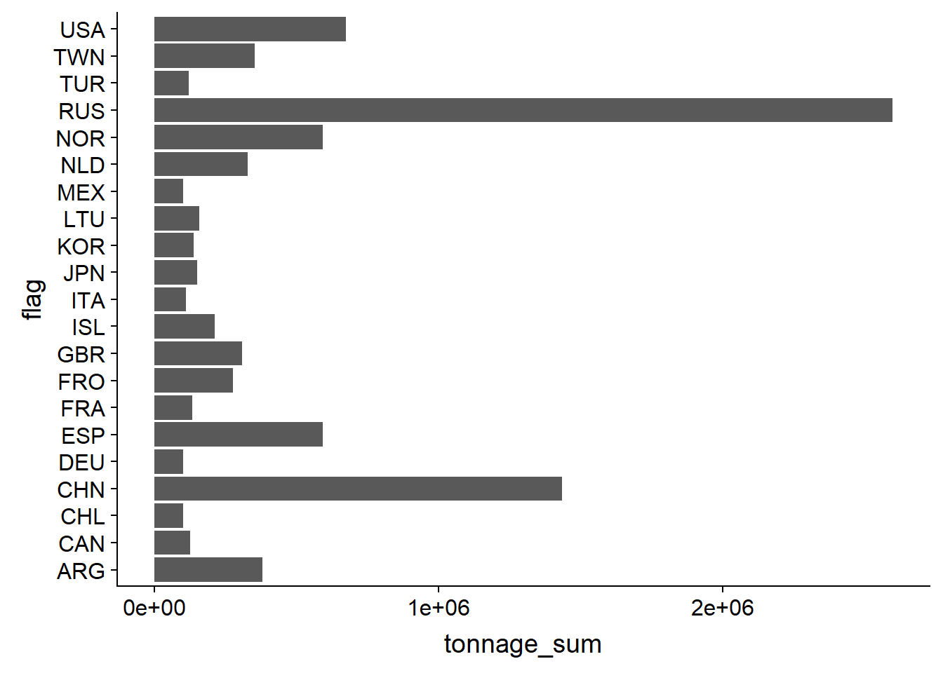
Using raw values distorts the data as larger countries will typically have a larger number of fishing vessels. Now we will normalise the tonnage data to map a chloropleth as a proportion, with the total tonnage per capita. GDP is already per capita available from the world dataset from Natural Earth, but we will also change to per million.
tonnage_prop <- left_join(vessels_world_sum,
                          world %>%
                                select(iso_a3, admin, pop_est, gdp_md_est) %>%
                                st_drop_geometry(),
                           by= c("flag"="iso_a3")) %>%
      mutate(tonnage_per_mil=(tonnage_sum/pop_est)*1000000) %>%
      mutate(gdp_per_mil=(gdp_md_est)/1000000)
Data Visualisation
Now we will create our final viz. With the new biscale R package that will classify the prepared data into mapping classes and add a bivariate legend, and a predefined bi_theme.
# Create mapping classes
bi_data <- bi_class(tonnage_prop, x = tonnage_per_mil, y = gdp_per_mil, style = "quantile", dim = 3)
# Create a legend with the per million of population abbreviation pmp
legend <- bi_legend(pal = "DkCyan",
                    dim = 3,
                    xlab = "Total Vessel Tonnage pmp",
                    ylab = "GDP pmp",
                    size = 8)
# Create a bivariate map
map <- ggplot() +
  geom_sf(data = bi_data %>%
                filter(bi_class !="NA-NA"),
          aes(fill = bi_class), color = "white", size = 0.1, show.legend = FALSE) +
  bi_scale_fill(pal = "DkCyan", dim = 3) +
  labs(x = NULL,
         y = NULL,
         title = "Global Fishing Vessels",
         subtitle= "For years 2012-2016",
         caption = "Data Sources:\n https://www.naturalearthdata.com/ \n https://globalfishingwatch.org/") +
  bi_theme()+
      theme(plot.caption = element_text(size = 12,hjust=0.75))
# combine map with legend
cowplot::ggdraw() +
  draw_plot(map, 0, 0, 1, 1) +
  draw_plot(legend, 0.1, .1, 0.2, 0.2)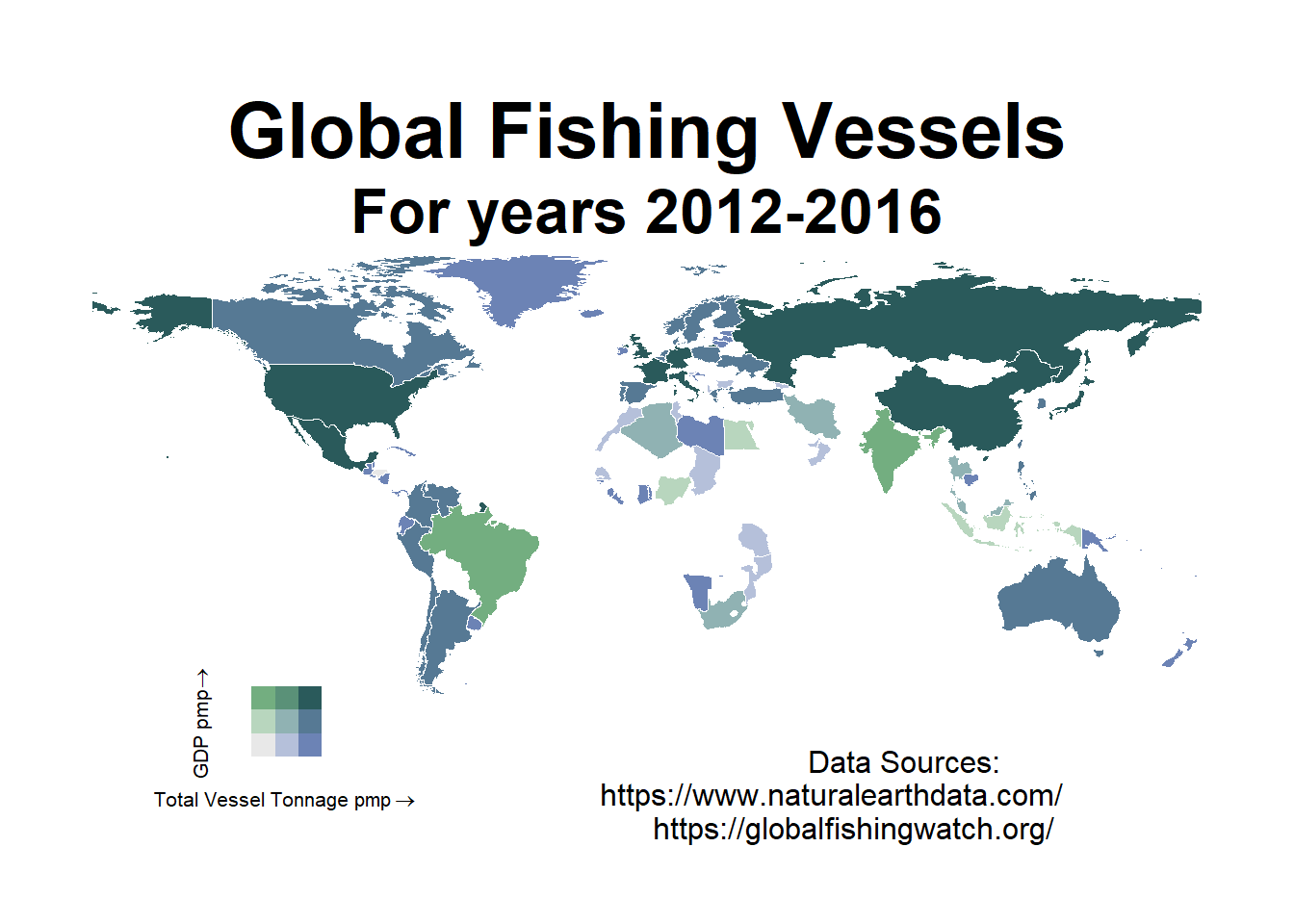
# Save ggplot for blogpost
# ggsave(filename = "vesselsmap.jpg") # default to last plot displayed
Conclusions
China, Great Britain, France, Spain and the USA appear to be big fishers. These big fishing developed countries are represented by the darker colour combination on the scale. Surprisingly, lower income countries such as Greenland, Botswana and Libya also have large fishing vessels fleets.
This is an initial view of big fisher countries who have the propensity to consume and or sell fish. It doesn’t however show in which waters they are actively fishing or what fish life are being caught. It could be useful to obtain shark numbers to see how many are being affected by fishing activities.
References
# Package citations as seen in freerangestats.info/blog/2019/03/30/afl-elo-adjusted
thankr::shoulders() %>%
  mutate(maintainer = str_squish(gsub("<.+>", "", maintainer))) %>%
  group_by(maintainer) %>%
  summarise(`Number packages` = sum(no_packages),
            packages = paste(packages, collapse = ", ")) %>%
knitr::kable() | maintainer | Number packages | packages |
|---|---|---|
| Achim Zeileis | 1 | colorspace |
| Andy South | 2 | rnaturalearth, rnaturalearthdata |
| Brian Ripley | 2 | class, KernSmooth |
| Brodie Gaslam | 1 | fansi |
| Charlotte Wickham | 1 | munsell |
| Christopher Prener | 1 | biscale |
| Claus O. Wilke | 1 | cowplot |
| David Meyer | 1 | e1071 |
| David Robinson | 1 | broom |
| Deepayan Sarkar | 1 | lattice |
| Dirk Eddelbuettel | 2 | digest, Rcpp |
| Edzer Pebesma | 3 | sf, sp, units |
| Gábor Csárdi | 3 | cli, crayon, pkgconfig |
| Hadley Wickham | 16 | assertthat, dplyr, forcats, ggplot2, gtable, haven, httr, lazyeval, modelr, plyr, rvest, scales, stringr, tidyr, tidyverse, vctrs |
| James Hester | 1 | xml2 |
| Jennifer Bryan | 2 | cellranger, readxl |
| Jeremy Stephens | 1 | yaml |
| Jeroen Ooms | 1 | jsonlite |
| Jim Hester | 3 | glue, withr, readr |
| Joe Cheng | 1 | htmltools |
| Justin Talbot | 1 | labeling |
| Kevin Ushey | 1 | rstudioapi |
| Kirill Müller | 4 | DBI, hms, pillar, tibble |
| Lionel Henry | 3 | purrr, rlang, tidyselect |
| Marek Gagolewski | 1 | stringi |
| Matt Dowle | 1 | data.table |
| Michel Lang | 1 | backports |
| Nathan Teetor | 1 | zeallot |
| Patrick O. Perry | 1 | utf8 |
| R-core | 1 | nlme |
| R Core Team | 10 | base, compiler, datasets, graphics, grDevices, grid, methods, stats, tools, utils |
| Roger Bivand | 2 | classInt, rgeos |
| Stefan Milton Bache | 1 | magrittr |
| Vitalie Spinu | 1 | lubridate |
| Winston Chang | 1 | R6 |
| Yihui Xie | 6 | blogdown, bookdown, evaluate, knitr, rmarkdown, xfun |