- Introduction
- Data
- Data Summary
- Exploratory Data Analysis
- Data Cleaning
- Data Visualisation
- Conclusions
- References
Introduction
We recently went swimming with sharks with a Marine Biologist. We asked the question “Is swimming with sharks dangerous?” in the dive brief about how to swim with sharks.
This is a spatial analysis of historical shark attacks.
# Load packages
library(tidyverse)
library(sf)
library(rnaturalearth)
Data
We will use the International Shark Attack File (ISAF) global shark attack csv dataset from 1580 until July 26, 2018.
url <- "https://www.engineeringbigdata.com/wp-content/uploads/global_shark_attacks.csv"
sharks <- read_csv(url)
## Parsed with column specification:
## cols(
## Country = col_character(),
## Total = col_integer()
## )Next retrieve the basemap data.
# Get the world sf dataset from rnaturalearth package
world <- ne_countries(scale = "medium", returnclass = "sf")
class(world)
## [1] "sf" "data.frame"# Join the basemap and sharks data
sharks_full <- left_join(sharks,world,by=c("Country"="name"))Data Summary
Let’s take a look at summary of the joined datasets.
# View the joined datasets by descending Totals
sharks_full %>%
      arrange(desc(Total))
## # A tibble: 90 x 65
## Country Total scalerank featurecla labelrank sovereignt sov_a3 adm0_dif
## <chr> <int> <int> <chr> <dbl> <chr> <chr> <dbl>
## 1 USA 1407 NA <NA> NA <NA> <NA> NA
## 2 Austra~ 621 1 Admin-0 c~ 2 Australia AU1 1
## 3 Republ~ 252 NA <NA> NA <NA> <NA> NA
## 4 Brazil 104 1 Admin-0 c~ 2 Brazil BRA 0
## 5 New Ze~ 51 1 Admin-0 c~ 2 New Zeala~ NZ1 1
## 6 Papua ~ 48 1 Admin-0 c~ 2 Papua New~ PNG 0
## 7 Mascar~ 42 NA <NA> NA <NA> <NA> NA
## 8 Mexico 40 1 Admin-0 c~ 2 Mexico MEX 0
## 9 Bahama~ 30 NA <NA> NA <NA> <NA> NA
## 10 Iran 23 1 Admin-0 c~ 2 Iran IRN 0
## # ... with 80 more rows, and 57 more variables: level <dbl>, type <chr>,
## # admin <chr>, adm0_a3 <chr>, geou_dif <dbl>, geounit <chr>,
## # gu_a3 <chr>, su_dif <dbl>, subunit <chr>, su_a3 <chr>, brk_diff <dbl>,
## # name_long <chr>, brk_a3 <chr>, brk_name <chr>, brk_group <chr>,
## # abbrev <chr>, postal <chr>, formal_en <chr>, formal_fr <chr>,
## # note_adm0 <chr>, note_brk <chr>, name_sort <chr>, name_alt <chr>,
## # mapcolor7 <dbl>, mapcolor8 <dbl>, mapcolor9 <dbl>, mapcolor13 <dbl>,
## # pop_est <dbl>, gdp_md_est <dbl>, pop_year <dbl>, lastcensus <dbl>,
## # gdp_year <dbl>, economy <chr>, income_grp <chr>, wikipedia <dbl>,
## # fips_10 <chr>, iso_a2 <chr>, iso_a3 <chr>, iso_n3 <chr>, un_a3 <chr>,
## # wb_a2 <chr>, wb_a3 <chr>, woe_id <dbl>, adm0_a3_is <chr>,
## # adm0_a3_us <chr>, adm0_a3_un <dbl>, adm0_a3_wb <dbl>, continent <chr>,
## # region_un <chr>, subregion <chr>, region_wb <chr>, name_len <dbl>,
## # long_len <dbl>, abbrev_len <dbl>, tiny <dbl>, homepart <dbl>,
## # geometry <MULTIPOLYGON [°]>It seems like some of the countries didn’t match up. Let’s extract the NA’s.
# Filter the NA countries from the join
sharks_full %>%
      filter(is.na(scalerank))
## # A tibble: 21 x 65
## Country Total scalerank featurecla labelrank sovereignt sov_a3 adm0_dif
## <chr> <int> <int> <chr> <dbl> <chr> <chr> <dbl>
## 1 USA 1407 NA <NA> NA <NA> <NA> NA
## 2 Republ~ 252 NA <NA> NA <NA> <NA> NA
## 3 Mascar~ 42 NA <NA> NA <NA> <NA> NA
## 4 Bahama~ 30 NA <NA> NA <NA> <NA> NA
## 5 Fiji I~ 22 NA <NA> NA <NA> <NA> NA
## 6 Solomo~ 11 NA <NA> NA <NA> <NA> NA
## 7 Marsha~ 8 NA <NA> NA <NA> <NA> NA
## 8 Canary~ 6 NA <NA> NA <NA> <NA> NA
## 9 French~ 5 NA <NA> NA <NA> <NA> NA
## 10 Federa~ 4 NA <NA> NA <NA> <NA> NA
## # ... with 11 more rows, and 57 more variables: level <dbl>, type <chr>,
## # admin <chr>, adm0_a3 <chr>, geou_dif <dbl>, geounit <chr>,
## # gu_a3 <chr>, su_dif <dbl>, subunit <chr>, su_a3 <chr>, brk_diff <dbl>,
## # name_long <chr>, brk_a3 <chr>, brk_name <chr>, brk_group <chr>,
## # abbrev <chr>, postal <chr>, formal_en <chr>, formal_fr <chr>,
## # note_adm0 <chr>, note_brk <chr>, name_sort <chr>, name_alt <chr>,
## # mapcolor7 <dbl>, mapcolor8 <dbl>, mapcolor9 <dbl>, mapcolor13 <dbl>,
## # pop_est <dbl>, gdp_md_est <dbl>, pop_year <dbl>, lastcensus <dbl>,
## # gdp_year <dbl>, economy <chr>, income_grp <chr>, wikipedia <dbl>,
## # fips_10 <chr>, iso_a2 <chr>, iso_a3 <chr>, iso_n3 <chr>, un_a3 <chr>,
## # wb_a2 <chr>, wb_a3 <chr>, woe_id <dbl>, adm0_a3_is <chr>,
## # adm0_a3_us <chr>, adm0_a3_un <dbl>, adm0_a3_wb <dbl>, continent <chr>,
## # region_un <chr>, subregion <chr>, region_wb <chr>, name_len <dbl>,
## # long_len <dbl>, abbrev_len <dbl>, tiny <dbl>, homepart <dbl>,
## # geometry <MULTIPOLYGON [°]>Data Cleaning
Use the stringr R package to clean the country names.
# Replace the mismatched country names where possible, create a new Country2 variable
sharks$Country2 <- sharks$Country %>%
      str_replace_all( c("USA"="United States",
                         "Republic of South Africa"="South Africa",
                         #"Mascarene Islands (Reunion Island)"= ,
                         "Bahama Islands"="Bahamas",
                         "Fiji Islands"="Fiji",
                         "Solomon Islands"="Solomon Is.",
                         "Marshall Islands"="Marshall Is.",
                         #"Canary Islands"=,
                         "French Polynesia"="Fr. Polynesia",
                         "Federated States of Micronesia"="Micronesia"))

# Join the sharks and world datasets again
sharks_full2 <- left_join(world,sharks,by=c("name"="Country2"))
# Check the class of this new jined object is sf
class(sharks_full2 )
## [1] "sf" "data.frame"Replace the NA Totals with 0 for the mapping.
# Replace the NA Totals  with 0
sharks_full2$Total <- sharks_full2$Total %>%
      replace_na(replace = 0)
Exploratory Data Analysis
Since the data are sf objects, we can use ggplot2 to create quick initial plots.
Sharks data
Let’s first take a look at the data using ggplot2.
 ggplot(data=sharks_full2)+
      geom_sf(aes(fill=Total))
This plot uses the default ggplot colour palette, which we will change to an oranges brewer palette with three breaks. We will also add labels to provide the context.
# Creat a ggplot map of the sharks dataset with labels, colours and breaks
 ggplot(data=sharks_full2)+
      geom_sf(aes(fill = cut_interval(sharks_full2$Total, 3)),
          color = NA) +
      scale_fill_brewer(palette = "Oranges")+
      labs(x = NULL,
         y = NULL,
         title = "Total Global Shark Attacks 1580 to 2018",
         caption = "Data Source: International Shark Attack File (ISAF) \n https://www.floridamuseum.ufl.edu/",
fill="Total") 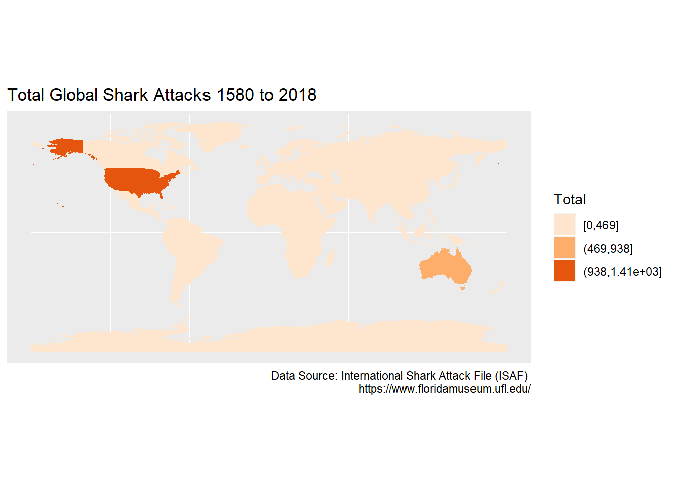
Let’s use the viridis R package for palette selection, and the lesser known cividis palette which ranges from a blue to yellow. See these colorspace charts for comparison.
# Creat a ggplot map of the sharks dataset with labels, colours and breaks
 ggplot(data=sharks_full2)+
      geom_sf(aes(fill = cut_interval(sharks_full2$Total, 4)),
          color = NA) +
      scale_fill_viridis_d(option = "cividis")+
      labs(x = NULL,
         y = NULL,
         title = "Total Global Shark Attacks 1580 to 2018",
         caption = "Data Source: International Shark Attack File (ISAF) \n https://www.floridamuseum.ufl.edu/",
fill="Total") 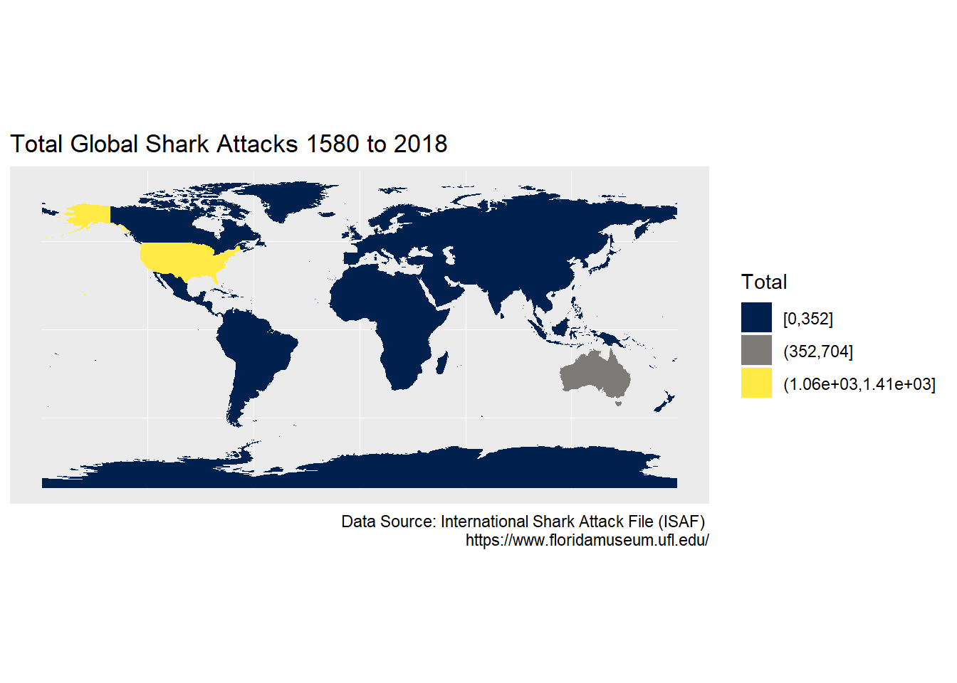
Three breaks doesn’t seem to be enough to capture the South African attacks. We will use four breaks in the final plot.
Data Visualisation
Now we will create our final viz. We will change the legend so that it looks neater with rounded four breaks on a single row on the bottom left. The theme will also be changed to a solid background to make it presentation quality.
# Creat a ggplot map of the dataset
g <- sharks_full2  %>%
  ggplot() +
    geom_sf(aes(fill=Total),color=NA) +
      labs(x = NULL,
         y = NULL,
         title = "Global Shark Attacks ",
         subtitle= "For years up to 2018",
         caption = "Data Source: International Shark Attack File (ISAF) \n https://www.floridamuseum.ufl.edu/") +
      # Dark background theme inspired by https://www.sharpsightlabs.com/blog/mapping-france-night/
    theme(text = element_text(family = "Gill Sans", color = "#E1E1E1"),
          plot.title = element_text(size = 18, color = "#E1E1E1",hjust = 0.5), # centre plot title
          plot.subtitle = element_text(size = 10,hjust = 0.5),
          plot.caption = element_text(size = 6),
          plot.background = element_rect(fill = "#000222"),
          panel.background = element_rect(fill = "#000222"),
          panel.grid.major = element_line(color = "#000222"),
          axis.text = element_blank(),
          axis.ticks = element_blank(),
          legend.background = element_blank(),
          legend.position = c(0.12, 0.32)
          )+
      # use the ggplot2 scale_fill_gradientn function as this sets the limits and a rounded interval rather than just splitting the range into 4 cut_interval. Extract the hex colours using the cividis function
    scale_fill_gradientn(colours = viridis::cividis(n=4),
                         limits=c(0,1500),
                         guide =   guide_legend( keyheight = unit(2, units = "mm"),
                                                 keywidth=unit(4, units = "mm"),
                                                 label.position = "bottom",
                                                 title.position = 'top',
                                                 nrow=1))
g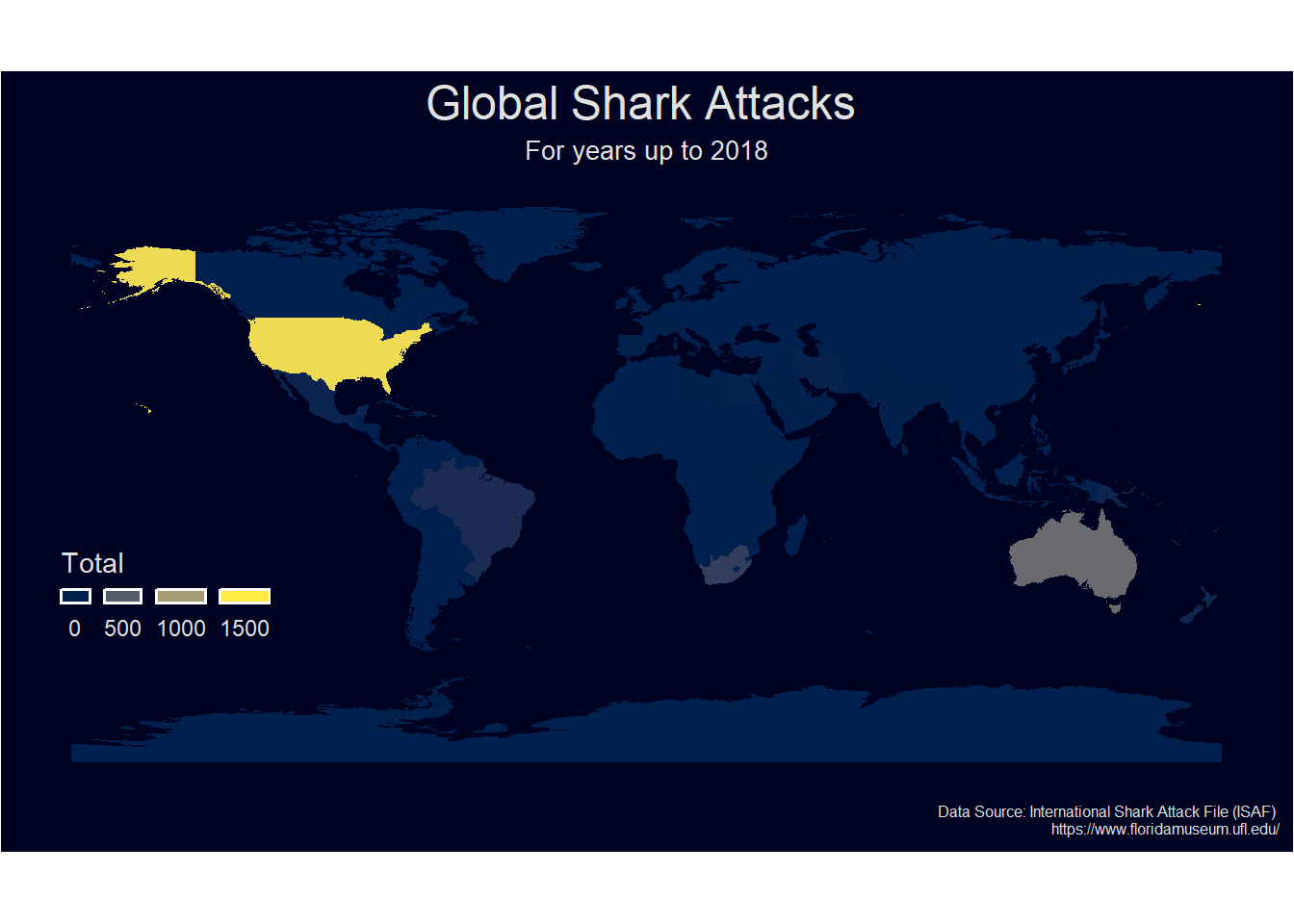
# Save ggplot for blogpost
# ggsave(filename = "sharksmap.jpg",g)
Conclusions
It turns out that people are more dangerous than sharks as historic reported shark numbers are much lower than one would expect from shark attack news reports.
According to to the Sustainable Ocean Society:
Sharks are apex predators, which help to keep a balance in the ocean, this balance has been created over millions of years of evolution. Sharks are under threat world wide.
References
# Package citations as seen in freerangestats.info/blog/2019/03/30/afl-elo-adjusted
thankr::shoulders() %>%
  mutate(maintainer = str_squish(gsub("<.+>", "", maintainer))) %>%
  group_by(maintainer) %>%
  summarise(`Number packages` = sum(no_packages),
            packages = paste(packages, collapse = ", ")) %>%
knitr::kable() | maintainer | Number packages | packages |
|---|---|---|
| Achim Zeileis | 1 | colorspace |
| Andy South | 2 | rnaturalearth, rnaturalearthdata |
| Baptiste Auguie | 1 | gridExtra |
| Brian Ripley | 1 | class |
| Brodie Gaslam | 1 | fansi |
| Charlotte Wickham | 1 | munsell |
| David Meyer | 1 | e1071 |
| David Robinson | 1 | broom |
| Deepayan Sarkar | 1 | lattice |
| Dirk Eddelbuettel | 2 | digest, Rcpp |
| Edzer Pebesma | 3 | sf, sp, units |
| Erich Neuwirth | 1 | RColorBrewer |
| Gábor Csárdi | 3 | cli, crayon, pkgconfig |
| Hadley Wickham | 15 | assertthat, dplyr, forcats, ggplot2, gtable, haven, httr, lazyeval, modelr, plyr, rvest, scales, stringr, tidyr, tidyverse |
| James Hester | 1 | xml2 |
| Jennifer Bryan | 2 | cellranger, readxl |
| Jeremy Stephens | 1 | yaml |
| Jeroen Ooms | 2 | curl, jsonlite |
| Jim Hester | 3 | glue, withr, readr |
| Joe Cheng | 1 | htmltools |
| Justin Talbot | 1 | labeling |
| Kevin Ushey | 1 | rstudioapi |
| Kirill Müller | 4 | DBI, hms, pillar, tibble |
| Lionel Henry | 3 | purrr, rlang, tidyselect |
| Marek Gagolewski | 1 | stringi |
| Michel Lang | 1 | backports |
| Patrick O. Perry | 1 | utf8 |
| R-core | 1 | nlme |
| R Core Team | 10 | base, compiler, datasets, graphics, grDevices, grid, methods, stats, tools, utils |
| Roger Bivand | 2 | classInt, rgeos |
| Simon Garnier | 2 | viridis, viridisLite |
| Stefan Milton Bache | 1 | magrittr |
| Vitalie Spinu | 1 | lubridate |
| Winston Chang | 1 | R6 |
| Yihui Xie | 6 | blogdown, bookdown, evaluate, knitr, rmarkdown, xfun |