- Introduction
- Import Data
- Data Summary
- Exploratory Data Analysis
- Data Cleaning
- Visualisations
- Conclusions
- References
Introduction
While touring the New Zealand South Island with friends in January 2019, one of our stops was the The University of Canterbury Mt John Observatory. Since it this area is a dark sky reserve, with a clear night and a new moon the midnight sky was lit up with stars and the milky way.
Inspired by our enthusiastic astrophysicist guide, Daniel, I thought that it would be relatively easy to replicate the evening sky chart in R and subsequently searched for R packages.
My initial searches (“plot the night sky rstats”) yielded no obvious results so I realised I had to learn some astronomical terminology.
According to Wikipedia in astronomy and navigation, the celestial sphere:
is an imaginary sphere of arbitrarily large radius, concentric with the observer. All objects in the observer’s sky can be thought of as projected upon the inside surface of the celestial sphere, as if it were the underside of a dome or a hemispherical screen.
This concept allows for visualising objects with no information of actual distances but objects appear to be on the sphere where the observer is appears to be still at the center.
So on Mt John we were observers looking at the night sky where the Earth
is at the center of the celestial sphere, an imaginary surface on which the planets, stars, and nebulae seem to be printed. On the celestial sphere, lines of right ascension and declination are similar to longitude and latitude lines on Earth.
Similar but different. Declination is also in degrees but right ascension is however a measure of time in hours.
I then changed my search to “celestial map” and came across Celestial map with D3.js. This website has some great demos and GeoJSON data sets where
For GeoJSON, all coordinates need to be given in degrees, longitude as [-180…180] deg, latitude as [-90…90] deg.
Phew. At this point I realised I could remain at astronomy level=curiosity and not have to study space time in order to produce a map.
I decided to attempt to create celestial maps in R using the sf R package as this package can both read in and plot spatial data with the ggplot.
Load Packages
library(tidyverse)
library(rnaturalearthdata)
library(rnaturalearth)
library(sf)
# install.packages("devtools")
# devtools::install_github("yutannihilation/ggsflabel")
Import Data
Earth data
We can get earth data from the rnaturalearth R package.
# Plot earth sphere using natural earth
earth <- ne_countries(scale = "medium", returnclass = "sf")
class(earth)
## [1] "sf" "data.frame"# Check the CRS of the earth
st_crs(earth)## Coordinate Reference System:
## EPSG: 4326
## proj4string: "+proj=longlat +datum=WGS84 +no_defs"# Create a sf point object for the Mt John Observatory
mtjohn <- st_point(c(170,-43)) %>% # create an sfg object ( a vector) with the geometry type POINT from the Mt John coordinates https://en.wikipedia.org/wiki/Mount_John_University_Observatory
st_sfc(crs=st_crs(earth)) %>% # convert to a geospatial sfc object ( a list) with CRS set to the same as the earth sf object
st_sf(name="Mt John Observatory") # Convert the geometry type POINT (a dataframe) with a CRS to an sf object and the point labelled with a nameCelestial data
Let’s read in the GeoJSON format celestial data using the sf R package.
I initially tried geojsonR and geojsonio R packages but sf reads in data as am sf object.
url1 <- "https://raw.githubusercontent.com/ofrohn/d3-celestial/master/data/constellations.lines.json"
# Read in the constellation lines data using the st_read function
constellation_lines_sf <- st_read(url1,stringsAsFactors = FALSE)
## Reading layer `constellations.lines' from data source `https://raw.githubusercontent.com/ofrohn/d3-celestial/master/data/constellations.lines.json' using driver `GeoJSON'
## Simple feature collection with 89 features and 1 field
## geometry type: MULTILINESTRING
## dimension: XY
## bbox: xmin: -177.9104 ymin: -83.6679 xmax: 179.9066 ymax: 89.2641
## epsg (SRID): 4326
## proj4string: +proj=longlat +datum=WGS84 +no_defsurl2 <- "https://raw.githubusercontent.com/ofrohn/d3-celestial/master/data/mw.json"
# Read in the milky way data using the st_read function
milky_sf <- st_read(url2,stringsAsFactors = FALSE)## Reading layer `mw' from data source `https://raw.githubusercontent.com/ofrohn/d3-celestial/master/data/mw.json' using driver `GeoJSON'
## Simple feature collection with 5 features and 1 field
## geometry type: MULTIPOLYGON
## dimension: XY
## bbox: xmin: -179.987 ymin: -74.9 xmax: 180 ymax: 66.946
## epsg (SRID): 4326
## proj4string: +proj=longlat +datum=WGS84 +no_defsurl3 <- "https://raw.githubusercontent.com/ofrohn/d3-celestial/master/data/stars.6.json"
# Read in the stars way data using the st_read function
stars_sf <- st_read(url3,stringsAsFactors = FALSE)## Reading layer `stars.6' from data source `https://raw.githubusercontent.com/ofrohn/d3-celestial/master/data/stars.6.json' using driver `GeoJSON'
## Simple feature collection with 4560 features and 5 fields
## geometry type: POINT
## dimension: XY
## bbox: xmin: -179.8148 ymin: -88.9565 xmax: 179.9871 ymax: 89.2641
## epsg (SRID): 4326
## proj4string: +proj=longlat +datum=WGS84 +no_defsThe planets data is not geojson
because positions need to be calculated by date from keplerian elements
So again, to remain a novice in this domain, we will not use planet data in this exercise.
Data Summary
Let’s take a look at the constellation_lines object.
# Use dplyr glimpse to view the data summary
glimpse(constellation_lines_sf)
## Observations: 89
## Variables: 2
## $ id <chr> "And", "Ant", "Aps", "Aqr", "Aql", "Ara", "Ari", "Aur...
## $ geometry <MULTILINESTRING [°]> MULTILINESTRING ((30.9748 4..., MULT...Let’s take a look at the milky_sf object.
# Use dplyr glimpse to view the data summary
glimpse(milky_sf)
## Observations: 5
## Variables: 2
## $ id <chr> "ol1", "ol2", "ol3", "ol4", "ol5"
## $ geometry <MULTIPOLYGON [°]> MULTIPOLYGON (((97.754 34.6..., MULTIPO...Let’s take a look at the stars_sf object.
# Use dplyr glimpse to view the data summary
glimpse(stars_sf)
## Observations: 4,560
## Variables: 6
## $ name <chr> "", "", "", "", "", "", "", "", "", "", "", "", "", "...
## $ desig <chr> "t", "HD224865", "<U+03B8>", "HD224893", "29", "30", "85", "...
## $ con <chr> "Phe", "", "Oct", "", "Psc", "Psc", "Peg", "Scl", "Ps...
## $ mag <dbl> 5.8690, 5.6243, 4.9354, 5.6725, 5.0831, 4.4120, 5.873...
## $ bv <chr> "0.911", "1.615", "1.254", "0.407", "-0.128", "1.631"...
## $ geometry <POINT [°]> POINT (0.2691 -48.8099), POINT (0.3338 -50.337...There are a large number of stars for a plot. We may need to filter the dataset in our plots.
Exploratory Data Analysis
Night Sky Theme for Plots
First create a custom theme function called theme_nightsky to use for all our plots.
# Use this custom function as a starting point to the format of the theme function https://jonlefcheck.net/2013/03/11/black-theme-for-ggplot2-2/

theme_nightsky <- function(base_size = 11, base_family = "") {

  theme_light(base_size = base_size, base_family = base_family) %+replace%
      theme(
      # Specify axis options, remove both axis titles and ticks but leave the text in white
      axis.title = element_blank(),
      axis.ticks = element_blank(),
      axis.text = element_text(colour = "white",size=6),
      # Specify legend options, here no legend is needed
      legend.position = "none",
      # Specify background of plotting area
      panel.grid.major = element_line(color = "grey35"),
      panel.grid.minor = element_line(color = "grey20"),
      panel.spacing = unit(0.5, "lines"),
      panel.background = element_rect(fill = "black", color  =  NA),
      panel.border = element_blank(),
      # Specify plot options
      plot.background = element_rect( fill = "black",color = "black"),
      plot.title = element_text(size = base_size*1.2, color = "white"),
      plot.margin = unit(rep(1, 4), "lines")
    )

}
Location of the Observatory
Let’s use this new theme to plot the earth data earth with the approximate location of the Mt John Observatory. We will keep the CRS of earth object as the default 4326, +proj=longlat +datum=WGS84 +no_defs. Use ggplot,sf and ggsflabel R package to label the sf geometry objects.
Although we have a theme, we still need to specify colours for the geoms. Additionally notice that the colour parameters are not included as aesthetics in the geom_sf code and the geom_sf function needs parameter data = included.
# Plot the earth using ggplot and sf
ggplot() +
      geom_sf(data = earth) +
      geom_sf(data = mtjohn,colour="yellow",size=2)+
      theme_nightsky()+
      ggsflabel::geom_sf_text_repel(data= mtjohn,
                   aes(label=mtjohn$name),
                   nudge_x = -1,
                   nudge_y=-1,
                   colour="yellow",
                   size=4)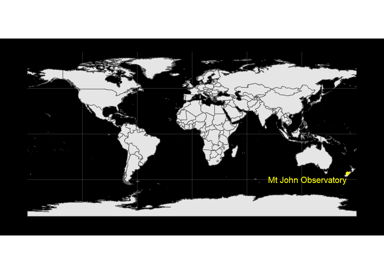
Milky way plot
Use ggplot to plot the milky_sf object which is a sfc_MULTIPOLYGON, sfc.
# Use ggplot to plot the milky way
milky_sf  %>%
      ggplot()+
      geom_sf()+
      theme_nightsky()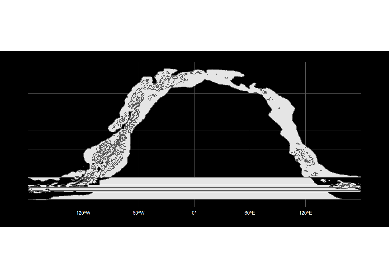
This plot has a few horizontal lines ?!? The polygons may be crossing -180 to 180 longitude.
Stars plot
Use ggplot to plot the stars_sf object which is a sfc_POINT, sfc. Incidently the brightest star has a negative magnitude value, which refers to apparent visual magnitude. We will need to convert this to a new newmag value in order to plot sizes to a scale from smallest to largest.
# Extract the constellation stars with names
stars_con_sf<- stars_sf %>%
      filter(name!="") %>%
      filter(con!="")
# Extract the brightest constellation stars with names, with an arbitrary cutoff 0.5 for mag - this extracts the top 10 brightest stars
stars_bright_sf<- stars_con_sf %>%
      filter(mag<0.5)
# Change the mag to a new scale newmag for the size aesthetic
stars_bright_sf<-stars_bright_sf %>%
      mutate(newmag=-(mag-1.1)/4)
# Use ggplot to plot the brighest stars by constellation
stars_bright_sf %>%
      ggplot()+
      # Group the stars by constellation
      geom_sf(aes(size=newmag,fill=con,colour=con))+
      geom_sf_text(aes(label=name), colour="white")+
      theme_nightsky()+
      # In this case add a legend to see the constellations and new magnitudes
      theme(legend.position="right")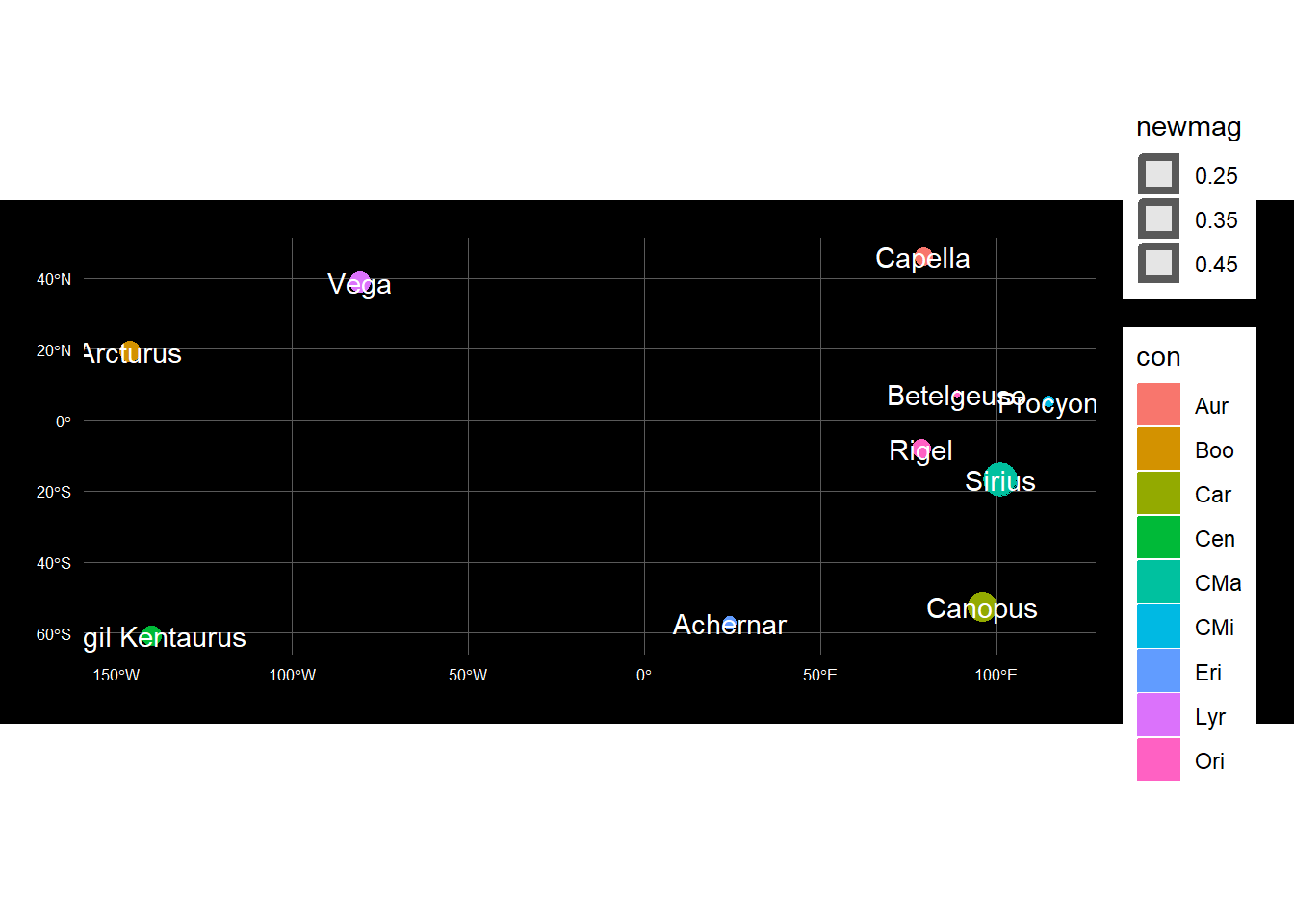
Constellation lines plot
Use ggplot to plot the constellation_lines_sf object which is a sfc_MULTILINESTRING, sfc.
# Use ggplot to plot the constellation lines
constellation_lines_sf %>%
      ggplot()+
      geom_sf(colour="white")+
      theme_nightsky()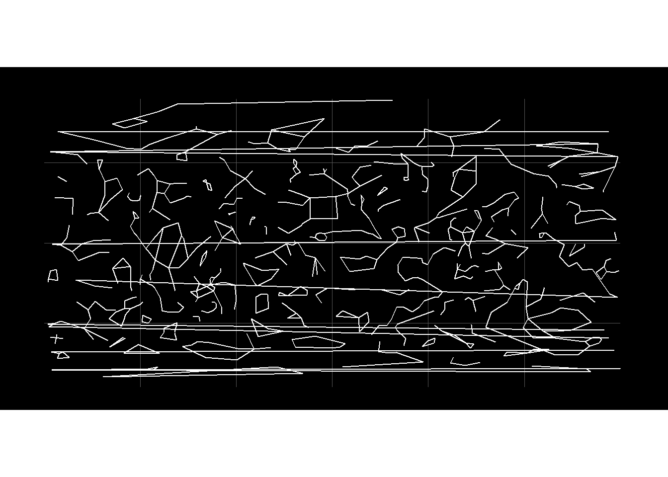
Again there are horizontal lines. We will look to clean the data to resolve the dateline issue in the next section.
Data Cleaning
Let’s look into ways to fix the horizontal lines.
Set Extent
Take a look at the Virgo Constellation, which has a horizontal line.
# Take a look at a constellation with a very broad range of longitudes
constellation_lines_sf %>%
      filter(id=="Vir") %>%
      ggplot()+
      geom_sf()+
      theme_nightsky()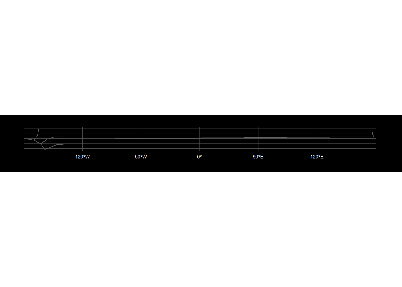
# Try to remove the lines by setting extent
 constellation_lines_sf %>%
      filter(id=="Vir") %>%
      ggplot()+
      geom_sf() +
      # Set the extent of the map using coord_sf
      coord_sf(xlim = c(-180,170),expand=FALSE)+
      theme_nightsky()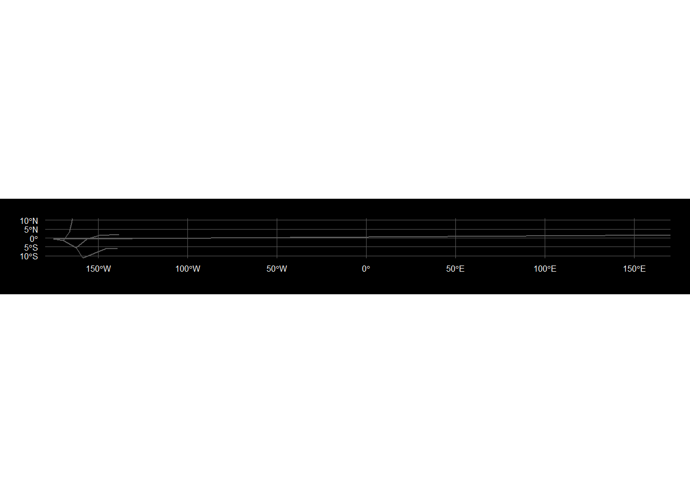
Although the extent has been reduced, there is still a horizontal line.
Crop the data sets
In order to crop the data, first convert the constellation lines data into points.
# Create points of the constellation lines
constellation_lines_sf_p <-constellation_lines_sf %>%
      # cast the MULTILINESTRING TO MULTIPOINT
      st_cast("MULTIPOINT")

# Create a table with the X,Y coordinates
(coords <- constellation_lines_sf_p %>%
      filter(id=="Vir") %>%
      st_coordinates() %>%
      as.data.frame() )
## X Y L1
## 1 176.4648 6.5294 1
## 2 177.6738 1.7647 1
## 3 -175.0235 -0.6668 1
## 4 -169.5848 -1.4494 1
## 5 -162.5125 -5.5390 1
## 6 -158.7018 -11.1613 1
## 7 -145.9964 -6.0005 1
## 8 -139.2349 -5.6582 1
## 9 -164.4558 10.9592 2
## 10 -166.0991 3.3975 2
## 11 -169.5848 -1.4494 2
## 12 -162.5125 -5.5390 3
## 13 -156.3267 -0.5958 3
## 14 -149.5884 1.5445 3
## 15 -138.4378 1.8929 3# Check the range of the coords
range(coords$X)## [1] -175.0235 177.6738range(coords$Y)## [1] -11.1613 10.9592# Plot the points of Virgo to visualise this new point geometry
constellation_lines_sf_p %>%
filter(id=="Vir") %>%
ggplot()+
geom_sf(colour="white") +
theme_nightsky()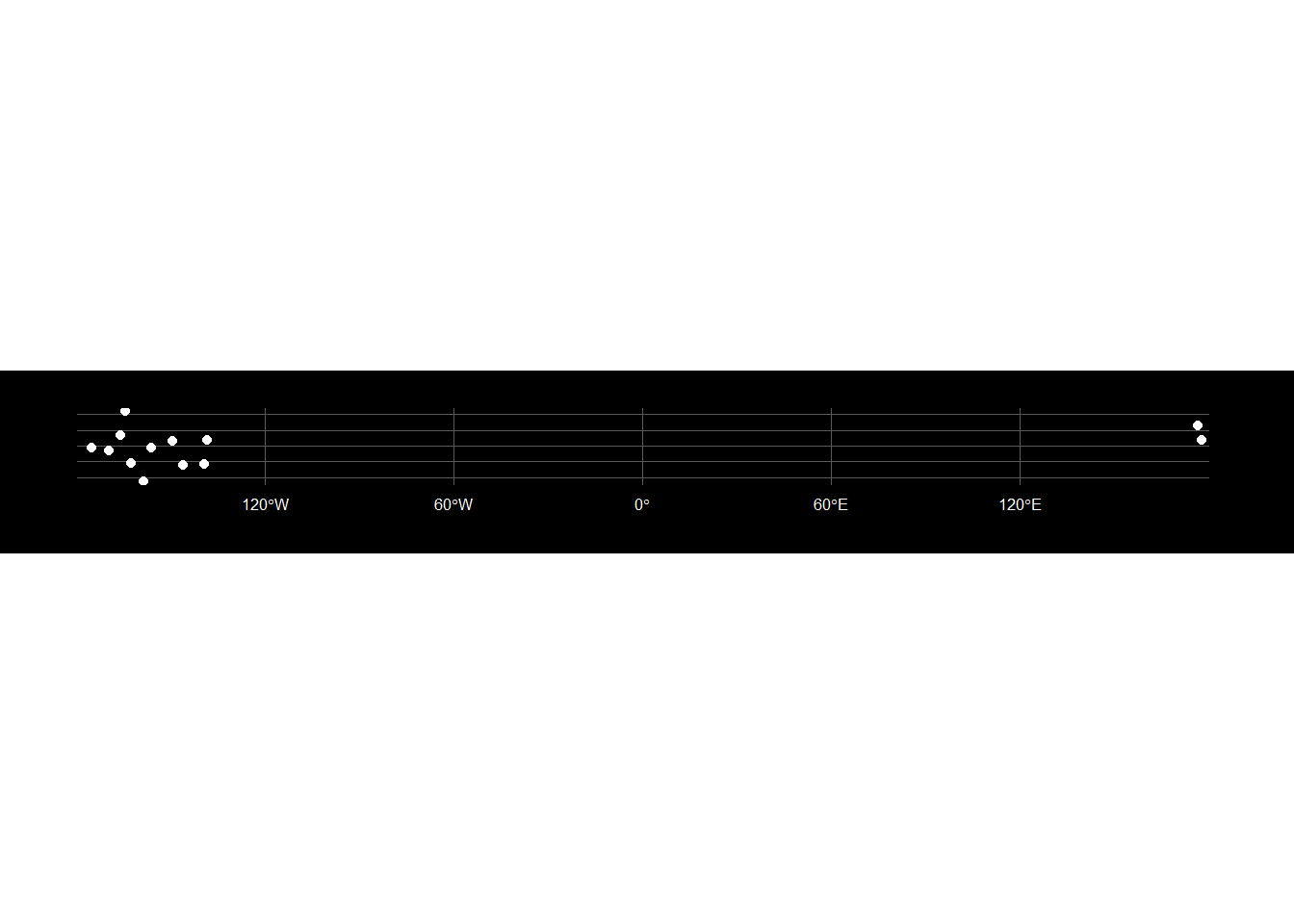
# Crop points then convert back to a MULTILINESTRING for one id Vir and visualise
constellation_lines_sf_p%>%
      filter(id=="Vir") %>%
#     https://github.com/r-spatial/sf/issues/720
      st_crop(xmin=-180,xmax=175,ymin=-180,ymax=180) %>%
      group_by( id )  %>%
      # Cast POINTS to LINESTRING
      st_cast("LINESTRING") %>%
      # Combine the LINESTRINGS into a single row as MULTILINESTRING sfc, however the id feature is now lost
      st_combine()  %>%
      ggplot()+
      geom_sf()+
      theme_nightsky()
## although coordinates are longitude/latitude, st_intersection assumes that they are planar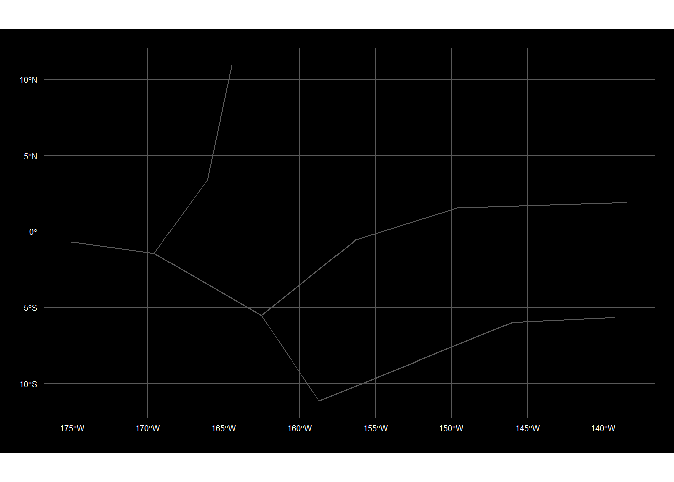
# Create a linestring function based on this example
to_linestring <- function(x)  st_cast(x,"LINESTRING") %>%
      st_combine() %>%  .[[1]]

# Crop the points based on and y min and max
constellation_lines_sf_cropped<-constellation_lines_sf_p %>%
      st_crop(xmin=-180,xmax=169,ymin=-180,ymax=180) %>%
      dplyr::group_by(id)%>%
      # Create a list of data variable using nest function https://www.r-spatial.org/r/2017/08/28/nest.html
      tidyr::nest()
## although coordinates are longitude/latitude, st_intersection assumes that they are planar# Convert the points to lines
newlines <- constellation_lines_sf_cropped %>%
# Since data is a list we cannot use select so use pull which is like [[ to extract the data variable list
pull(data) %>%
map(to_linestring) %>%
st_sfc(crs = st_crs(earth))
# This error came up as we tried to run the function on the cropped data:Error in st_cast.POINT(X[[i]], ...) : cannot create LINESTRING from POINT. Turns out the function was creating single points which could not be cast to lines
constellation_lines_sf_new <- constellation_lines_sf_cropped %>%
select(-data) %>%
st_sf(geometry = newlines)
# Plot cropped constellation lines
constellation_lines_sf_new %>%
ggplot()+
geom_sf()+
theme_nightsky()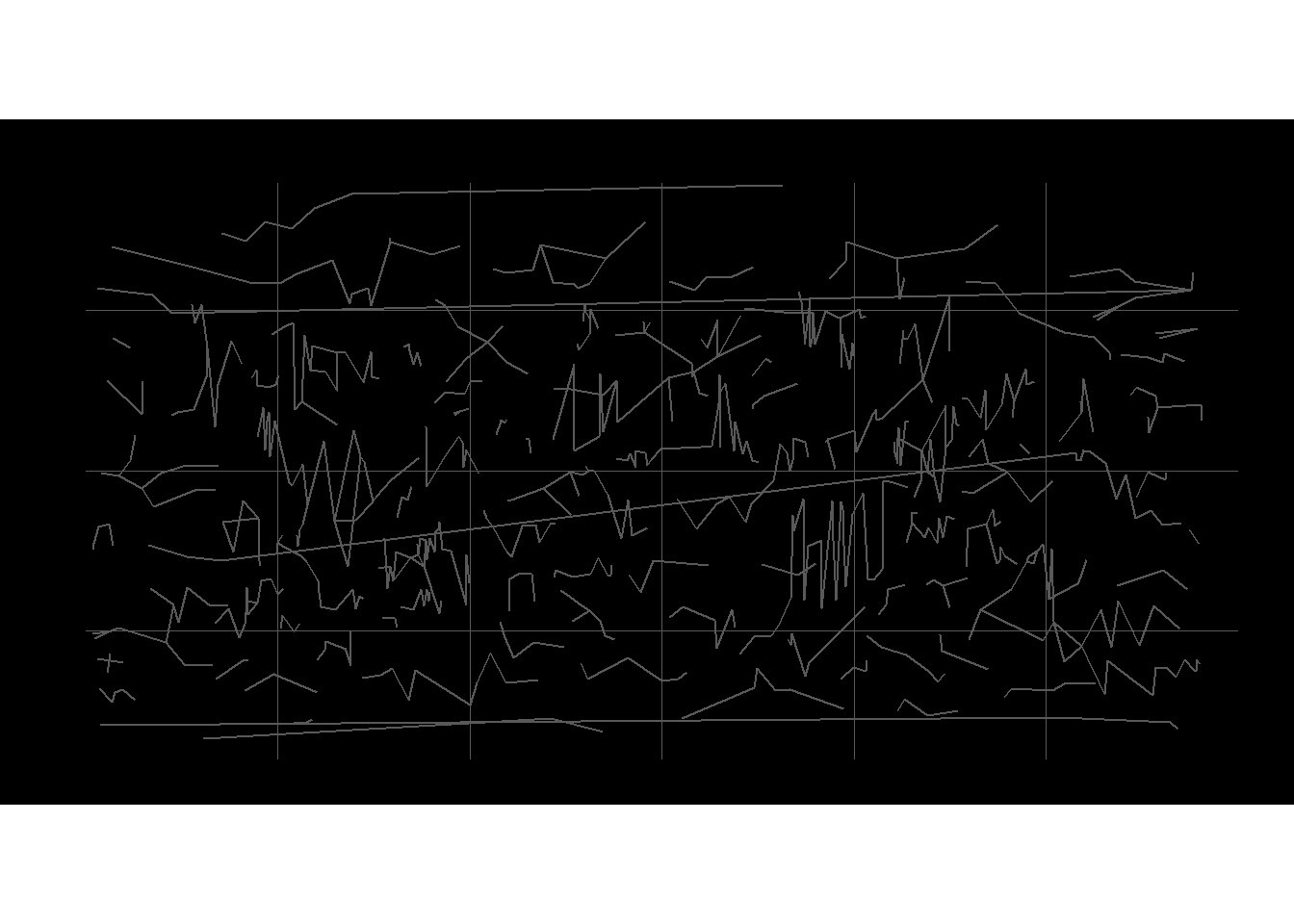
The Virgo constellation has been cropped and now doesn’t have the horizontal line. However some other constellations still have the lines.
This data cleaning method has a couple of downsides.It removes data creating data quality issues, for example if the globe is rotated then there would be lines missing and it is time intensive manual process.
Let’s look for a different approach.
Coordinate Analysis
Let’s extract and analyse the coordinates of the horizontal lines in milky_sf that are creating the unexpected horizontal lines.
# Extract the coordinates from the milk_sf object
milkycoords <- milky_sf %>%
      st_coordinates() %>%
      as.data.frame()

# Identify the coordinates where the X coordinate has crossed from + to - or from - to +
firstX <- milkycoords[1,1]
(milkycoords_cross <- milkycoords %>%
      mutate(prevXval=ifelse(X!=firstX,lag(X),0)) %>%
      mutate(prevYval=ifelse(X!=firstX,lag(Y),0))%>%
      mutate(prevL1=ifelse(X!=firstX,lag(L1),0))%>%
      mutate(cross=ifelse(L1!=prevL1,"NOCROSS", # check diff L1 object first
            ifelse(prevXval>0, ifelse(X>0,"NOCROSS", # X and prevval pos
                  "CROSS"), # X is pos and prevval is neg
                  ifelse(X<0,"NOCROSS",  # X and prevval both neg
                        "CROSS") ))) %>% # X is neg and prevval pos
      select(-L1,-L2,-L3,-prevL1) %>%
      filter(cross=="CROSS") %>%
      select(-cross) )
## X Y prevXval prevYval
## 1 -0.121 65.001 0.067 65.117
## 2 180.000 -50.039 -179.879 -50.156
## 3 -0.075 47.787 0.038 47.904
## 4 179.754 -73.960 -179.900 -73.979
## 5 -0.012 60.529 0.146 60.646
## 6 0.092 63.999 -0.133 63.981
## 7 -179.929 -58.704 179.883 -58.686
## 8 179.846 -66.118 -179.958 -66.236
## 9 -179.742 -65.234 179.979 -65.314
## 10 179.783 -64.687 -179.987 -64.706
## 11 -179.842 -61.156 179.992 -61.039
## 12 179.867 -63.981 -179.867 -63.901# Create a function that creates a linestring that extracts vectors (using the as.numeric fn) of the X,Y and prevXval, prevYval points from nx4 dataframe, then bind to a matrix
make_line <- function(x) {rbind(as.numeric(milkycoords_cross[x,1:2]),
as.numeric(milkycoords_cross[x,3:4]))%>%
# Convert to a linestring object
st_linestring() %>%
st_sfc(crs=st_crs(earth)) %>%
# Convert to a geospatial sfc object ( a list) with CRS set to the same as the earth sf object
st_sf()
}
# Check function works on the first set of points
make_line(1)## Simple feature collection with 1 feature and 0 fields
## geometry type: LINESTRING
## dimension: XY
## bbox: xmin: -0.121 ymin: 65.001 xmax: 0.067 ymax: 65.117
## epsg (SRID): 4326
## proj4string: +proj=longlat +datum=WGS84 +no_defs
## geometry
## 1 LINESTRING (-0.121 65.001, ...# I could not find a way to get the function to apply over rows so I posted this question https://gis.stackexchange.com/questions/312289/r-create-multiple-linestrings-from-multiple-coordinates
# The key here was to use matrix functionality to reshape the coordinates and then convert the dataframe rows into a list so that purrr could iterate over the list
# Now create an sf object with all the lines
milkyhorizlines_sf <- map(split(milkycoords_cross, seq(nrow(milkycoords_cross))), function(row) {
matrix(unlist(row[1:4]), ncol = 2, byrow = TRUE) %>%
st_linestring()
}) %>%
st_sfc(crs=st_crs(earth)) %>%
st_sf() %>%
# Cast to MULTILINESTRING to avoid Error in CPL_geos_is_empty(st_geometry(x)) :
st_cast("MULTILINESTRING")
# Plot the horizontal lines only
milkyhorizlines_sf %>%
ggplot()+
geom_sf()+
theme_nightsky()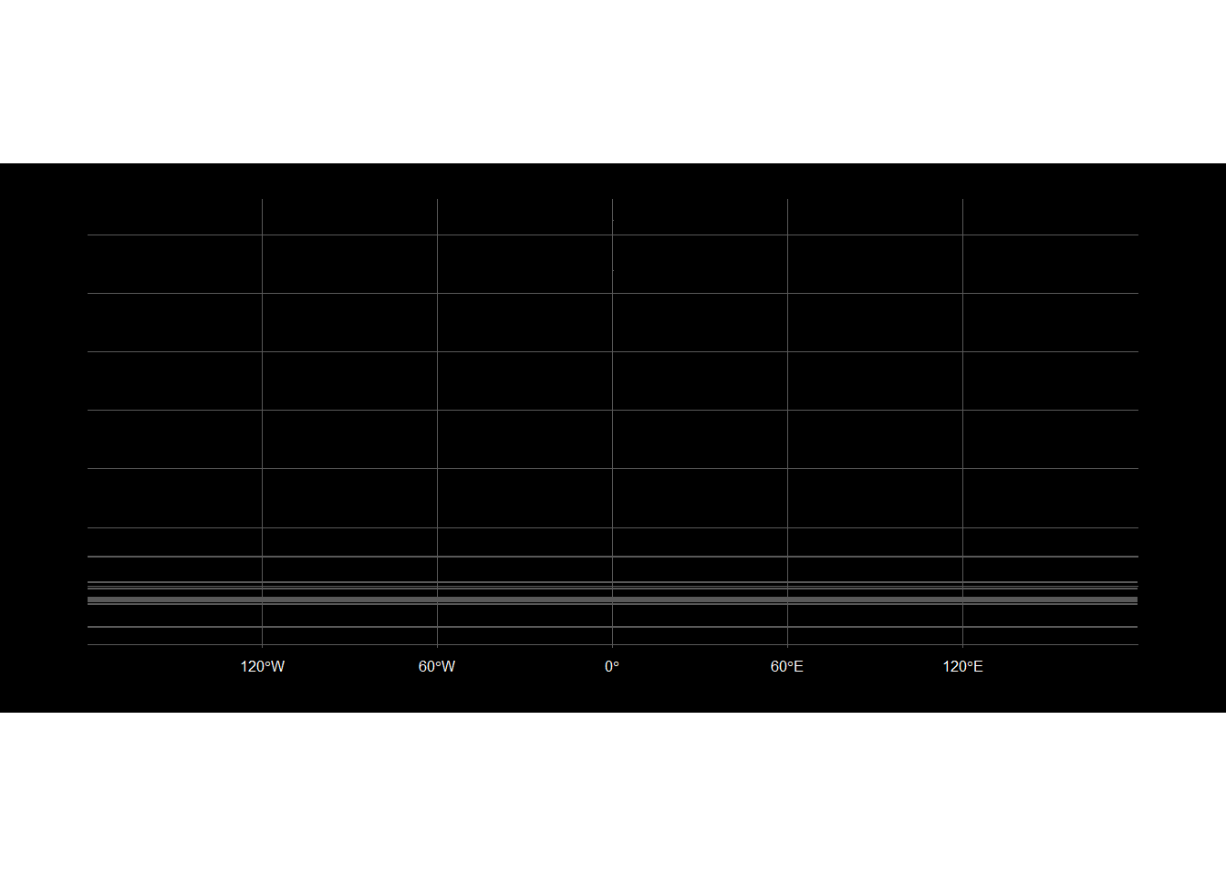
Potentially the milkyhorizlines_sf could be plotted over in black to hide the lines. However this would work for lines however it may not work with polygons if they are filled.
Wrap Date Line
There is also an sf function st_wrap_dateline to transform a polygon that crosses the dateline. This appears to be the better approach as there is no potential data removal and it involves a simpler function to the previous approaches.
# Try to remove the lines by st_wrap_dateline function
 constellation_lines_sf %>%
  st_wrap_dateline(options = c("WRAPDATELINE=YES", "DATELINEOFFSET=180"))%>%
      ggplot()+
      geom_sf()+
      theme_nightsky()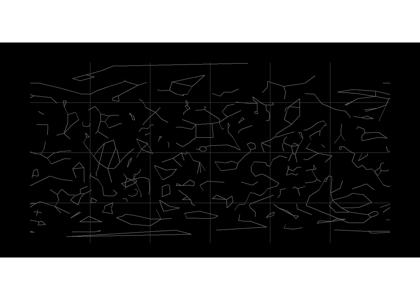
This appears to work for the constellation lines so we will use a transformed object in the final plot for constellation_lines.
# Transform the  constellation_lines_sf
constellation_lines_sf_trans <- constellation_lines_sf %>%
  st_wrap_dateline(options = c("WRAPDATELINE=YES", "DATELINEOFFSET=180")) %>%
      st_cast("MULTILINESTRING")
Let’s apply this function to the milky_sf object.
# Try to remove the lines by st_wrap_dateline function
milky_sf  %>%
      st_cast("MULTILINESTRING") %>%
  st_wrap_dateline(options = c("WRAPDATELINE=YES", "DATELINEOFFSET=0")) %>%
      ggplot()+
      geom_sf()+
      theme_nightsky()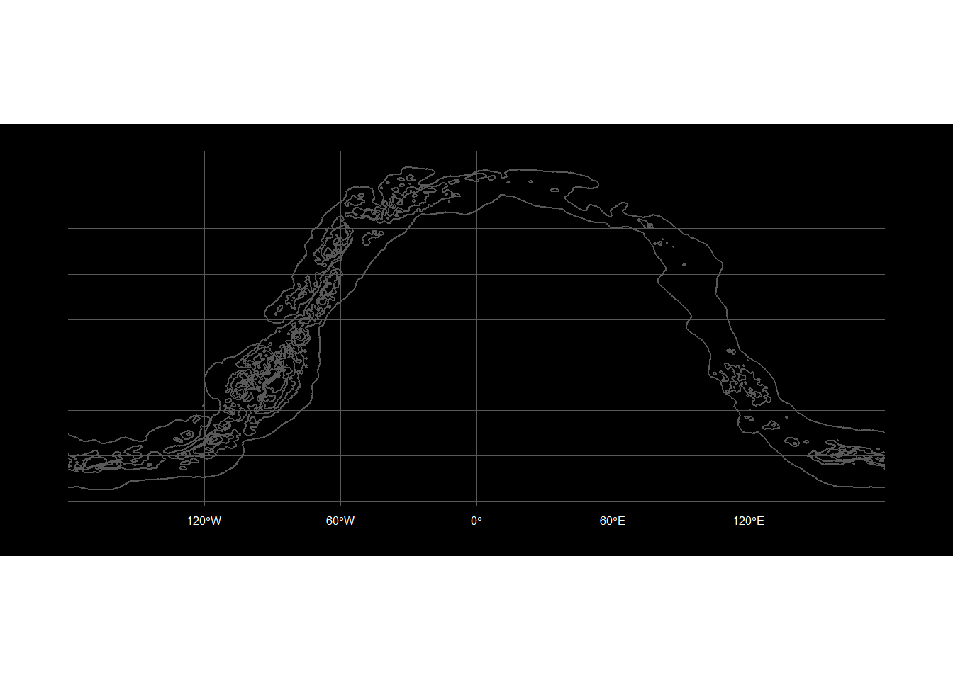
This appears to work for the milky_sf so we will use a transformed object in the final plot.
# Transform milky_sf with st_wrap_dateline
milky_sf_trans <- milky_sf %>%
      # These polygons have errrors with the st_wrap_dateline so add a cast to MULTILINESTRING then LINESTRING to break it up smaller
       st_cast("MULTILINESTRING") %>%
       st_cast("LINESTRING") %>%
       group_by(id)%>%
       st_wrap_dateline(options = c("WRAPDATELINE=YES", "DATELINEOFFSET=180"))

# Convert the milky way back to MULTIPOLYGON so it will fill with grey in the plots, the outer od1 lines are on the 180 and -180 so we need to treat these separately using  to the other lines which we can convert to MULTIPOLYGON
milky_sf_trans[3:202,]<- milky_sf_trans[3:202,] %>%
      st_cast("MULTIPOLYGON")
# Use concaveman R package https://github.com/joelgombin/concaveman or https://gis.stackexchange.com/questions/290170/convert-a-linestring-into-a-closed-polygon-when-the-points-are-not-in-order to create a polygon of the outer milky way
milky_sf_transclosed <- concaveman::concaveman(milky_sf_trans[1:2,])
# Now plot these transformed objects to check
ggplot() +
     geom_sf(data = milky_sf_transclosed,alpha=0.9,aes(fill=id))+
     geom_sf(data = milky_sf_trans,alpha=0.4,aes(fill=id)) +
     # Fill the milky way - inversely plot the discrete polygon values from light grey in the center
      scale_fill_grey()+
theme_nightsky()![]()
Reprojecting the CRS
Since we are mapping the night sky let’s find an ellipsoidal projection rather than the default projection 4326, +proj=longlat +datum=WGS84 +no_defs. Reviewing the excellent Geocomputation for R, we discover the Mollweide projection preserves area relationships and one of its applications is global maps of the night sky. An alternative is the Aitoff projection but this creates a GDAL error in st_transform() so it does not appear available with sf at the moment.
# Check the CRS of the stars, constellation and milky way objects
st_crs(stars_sf)
## Coordinate Reference System:
## EPSG: 4326
## proj4string: "+proj=longlat +datum=WGS84 +no_defs"st_crs(stars_bright_sf)## Coordinate Reference System:
## EPSG: 4326
## proj4string: "+proj=longlat +datum=WGS84 +no_defs"st_crs(constellation_lines_sf_trans)## Coordinate Reference System:
## EPSG: 4326
## proj4string: "+proj=longlat +datum=WGS84 +no_defs"st_crs(milky_sf_trans)## Coordinate Reference System:
## EPSG: 4326
## proj4string: "+proj=longlat +datum=WGS84 +no_defs"st_crs(milky_sf_transclosed)## Coordinate Reference System:
## EPSG: 4326
## proj4string: "+proj=longlat +datum=WGS84 +no_defs"The star maps objects have been loaded with CRS 4326, +proj=longlat +datum=WGS84 +no_defs, the same CRS 4326, +proj=longlat +datum=WGS84 +no_defs as the earth object.
# Transform stars_sf to Mollweide CRS
stars_sf<- st_transform(stars_sf, crs = "+proj=moll")

# Transform stars_bright_sf to Mollweide CRS
stars_bright_sf<- st_transform(stars_bright_sf, crs = "+proj=moll")

# Transform constellation_lines_sf_trans to Mollweide CRS
constellation_lines_sf_trans<- st_transform(constellation_lines_sf_trans, crs = "+proj=moll")

# Transform milky_sf_trans to Mollweide CRS
milky_sf_trans<- st_transform(milky_sf_trans, crs = "+proj=moll")

# Transform milky_sf_trans to Mollweide CRS
milky_sf_transclosed<- st_transform(milky_sf_transclosed, crs = "+proj=moll")

# Let's take a look at the new CRS of one of the objects
st_crs(milky_sf_trans)
## Coordinate Reference System:
## No EPSG code
## proj4string: "+proj=moll +lon_0=0 +x_0=0 +y_0=0 +ellps=WGS84 +units=m +no_defs"Visualisations
10 Brightest Stars
Since the number of objects in the universe is so large,to create a plot as introductory first look at a celestial map, let’s first take a look at the 10 brightest stars. Use ggplot and sf R packages.
We will start with a simplified plot of the 10 brightest stars to minimise cognitive load on a person looking at a celestial map for the first time. Although stars can be different colours but this subject itself is too complex to explain in one plot. We will therefore use our black and white theme“. For the plot colours, use different greys to soften the contrast of black and white. The sizing of the stars is not to scale but they provide an idea of size and positioning relative to each other. The other constellation stars are plotted as small white dots on a globe with graticules to provide further visual clues that this is a star map. The tooltips provide information on the star name, magnitude and constellation to encourage further research or reading.
First create the ggplot object.
# Create a ggplot object and use the hover text functionality.
(starplot1 <- ggplot() +
      geom_sf(data = milky_sf_transclosed,
              alpha=0.2,
              aes(fill=id))+
      geom_sf(data = milky_sf_trans,
              alpha=0.4,
              aes(fill=id)) +
      # Plot the constellation stars  as small white dots
      geom_sf(data=stars_sf,
              colour="grey60",
              size=0.2) +
      # Now plot the bright stars
      geom_sf(data=stars_bright_sf,
              colour="grey88",
              aes(size=stars_bright_sf$newmag,
                  text=paste('</br>Name: ',name,'</br>Stellar Magnitude: ',mag,'</br>Constellation: ',con)))  +
      # Fill the milky way - inversely plot the discrete polygon values from light grey in the center
      scale_fill_grey()+
      theme_nightsky()+
      ggtitle("The 10 Brightest Stars") )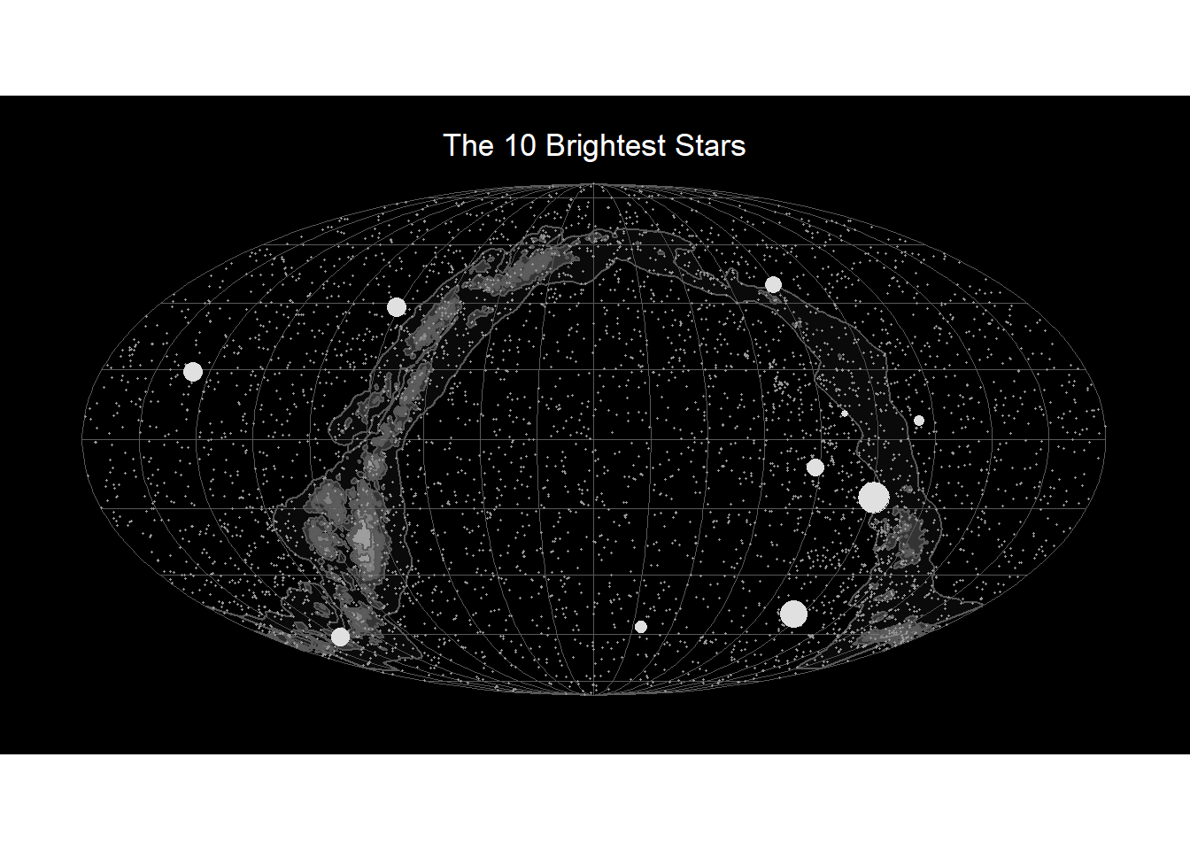
# Now add the labels with star names
(starplot1_labels <- starplot1 +
      ggsflabel::geom_sf_text_repel(data= stars_bright_sf,
                   aes(label=stars_bright_sf$name),
                        nudge_x = -2,
                   colour="white",
                   size=2.5))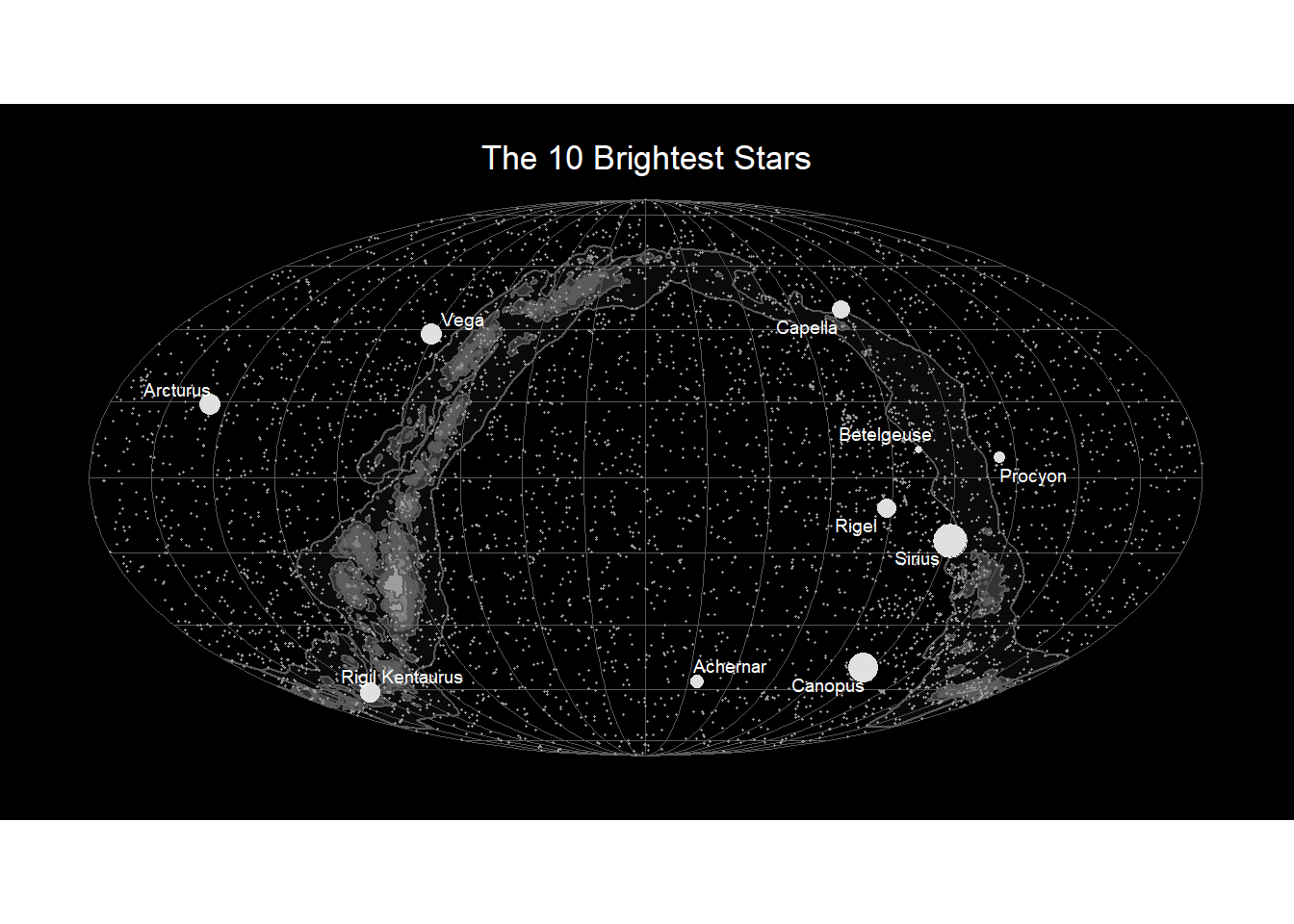
# Save ggplot for blog post
# ggsave("starplot1_labels.jpg",starplot1_labels)
Celestial Map with More objects
Now use ggplot, sf and ggsflabel again to plot a star map with more objects for someone who would like to know more about the sky, including the constellations. This time we use other colours to label the objects as this one is a lot busier.
# Plot the stars,constellations and milky way with a starplot ggplot object.
starplot2<- ggplot() +
     geom_sf(data = milky_sf_trans,alpha=0.4,aes(fill=id)) +
     # Fill the milky way - inversely plot the discrete polygon values from light grey in the center
      scale_fill_grey()+
      # Plot the consteallation stars as small white dots. Stars actually have different colours white, red etc but in this case we will keep to ablack and white theme
      geom_sf( data=stars_sf, colour="lightgrey",size=0.1) +
      # Now plot the bright stars
      geom_sf(data=stars_bright_sf,  colour="white", aes(size=stars_bright_sf$newmag) ) +
      geom_sf(data =constellation_lines_sf_trans, alpha=0.2, colour="lightgrey")  +
      theme_nightsky()+
      ggtitle("Constellations, Stars and the Milky Way")
# Plot the starplot2 with the labels
starplot2+
      ggsflabel::geom_sf_text_repel(data= stars_bright_sf,
                   aes(label=stars_bright_sf$name),
                        nudge_x = -2,
                   colour="yellow",
                   size=2.5)+
     ggsflabel::geom_sf_text_repel(data= constellation_lines_sf,
                   aes(label=constellation_lines_sf$id),
                        nudge_x = -1,
                   colour="lightblue",
                   size=2)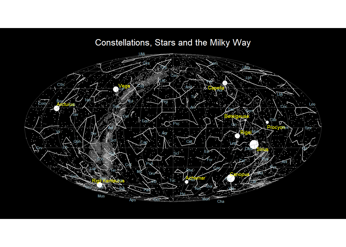
Conclusions
From the tour and subsequently analysing this data, here are some things I learnt about the stars:
- Sirius is the brightest star in the constellation Canis Major, a white dwarf and is commonly know as the Dog Star, followed by the second brightest star, Canopus.
- Alpha Centauri is also known as Rigel Kentaurus, and actually a system of three stars Alpha Centauri A, Alpha Centauri B and Alpha Centauri C.
- In stellar apparent visual magnitude, the brighter objects have higher negative numbers and the fainter have higher positive numbers.
This exercise involved more data manipulation than I expected but it has been great data structure thinking practice.
Packages like sf and purrr use lists and it is often a good solution to a problem to convert data into a list first, then iterate over the list. This can be done with functions like nest and split. Additionally matrix functionality can be used to reshape a dataframe.
Although I spent a LOT of time thinking thinking through the dateline issue, I discovered the st_wrap_dateline which is a great addition to the toolkit for the next horizontal lines issue.
Other Tools for Sky Maps
Here are some other tools to produce planetarium type looking up at the sky maps.
References
- d3-celestial data includes citations to source data.
- Geocomputation for R
- The Ten Brightest Stars in the Sky
- Stellar magnitude