- Introduction
- Data Overview
- Load Data
- Data Cleaning
- Exploratory Data Analysis
- Animation
- Conclusions
- References
Introduction
I went to my first basketball game on 27 January 2019 to watch the Skycity Breakers versus Brisbane Bullets. The final score was Breakers 109-96 Bullets.
Since it was a close game I wondered if the type of shots attempted got closer to the hoop under pressure near the end of time, assuming that shorter range shots have a better success rate ?
This is an analysis of basketball data and experimentation with the updated gganimate R package.
library(tidyverse)## -- Attaching packages ----------------------------------------------- tidyverse 1.2.1 --## v ggplot2 3.1.0 v purrr 0.2.5
## v tibble 2.0.1 v dplyr 0.7.6
## v tidyr 0.8.1 v stringr 1.4.0
## v readr 1.1.1 v forcats 0.3.0## Warning: package 'ggplot2' was built under R version 3.5.2## Warning: package 'tibble' was built under R version 3.5.2## Warning: package 'stringr' was built under R version 3.5.2## -- Conflicts -------------------------------------------------- tidyverse_conflicts() --
## x dplyr::filter() masks stats::filter()
## x dplyr::lag() masks stats::lag()library(gganimate)## Warning: package 'gganimate' was built under R version 3.5.2Data Overview
There are some stats available on the Breakers and NBL websites however it would require time and effort to web scrape. There is also shots data in csv format available from Andrew Price’s GitHib which we will use. The downside is that this was published in 2016, so covering recent data from Sunday’s game but it will serve the purpose of a first attempt at analysing Breakers data.
Load Data
First import the data using readr R package.
url <-  "https://raw.githubusercontent.com/andrewbprice/NBLShotCharts-D3/master/combinedShots_all.csv"
shots <- read_csv(url)
## Parsed with column specification:
## cols(
## J = col_integer(),
## Team = col_character(),
## teamScore = col_integer(),
## opponent = col_character(),
## opponentScore = col_integer(),
## Home = col_integer(),
## Player = col_character(),
## PlayerNo = col_integer(),
## X = col_double(),
## Y = col_double(),
## ShotType = col_character(),
## SubType = col_character(),
## Result = col_integer(),
## Quarter = col_integer(),
## `Game #` = col_integer(),
## Season = col_character(),
## League = col_character()
## )# View a summary statistics f the data
skimr::skim(shots)## Skim summary statistics
## n obs: 81371
## n variables: 17
##
## -- Variable type:character -------------------------------------------------------------
## variable missing complete n min max empty n_unique
## League 0 81371 81371 3 6 0 4
## opponent 0 81371 81371 6 27 0 43
## Player 0 81371 81371 5 19 0 610
## Season 0 81371 81371 8 22 0 8
## ShotType 0 81371 81371 3 3 0 2
## SubType 26532 54839 81371 4 8 0 5
## Team 0 81371 81371 6 27 0 43
##
## -- Variable type:integer ---------------------------------------------------------------
## variable missing complete n mean sd p0 p25
## Game # 0 81371 81371 26814.76 65402.84 1 33
## Home 0 81371 81371 0.5 0.5 0 0
## J 0 81371 81371 235173.54 75818.41 137220 139044
## opponentScore 0 81371 81371 83.29 12.94 11 74
## PlayerNo 0 81371 81371 7.66 4.4 1 4
## Quarter 434 80937 81371 2.48 1.12 1 1
## Result 0 81371 81371 0.44 0.5 0 0
## teamScore 0 81371 81371 83.52 12.98 11 74
## p50 p75 p100 hist
## 72 142 238958 <U+2587><U+2581><U+2581><U+2581><U+2581><U+2581><U+2581><U+2581>
## 1 1 1 <U+2587><U+2581><U+2581><U+2581><U+2581><U+2581><U+2581><U+2587>
## 281624 281768 377959 <U+2586><U+2581><U+2581><U+2581><U+2587><U+2582><U+2581><U+2581>
## 84 92 133 <U+2581><U+2581><U+2581><U+2583><U+2587><U+2586><U+2581><U+2581>
## 7 11 23 <U+2587><U+2587><U+2587><U+2587><U+2583><U+2582><U+2581><U+2581>
## 2 3 4 <U+2587><U+2581><U+2587><U+2581><U+2581><U+2587><U+2581><U+2587>
## 0 1 1 <U+2587><U+2581><U+2581><U+2581><U+2581><U+2581><U+2581><U+2586>
## 84 92 133 <U+2581><U+2581><U+2581><U+2583><U+2587><U+2586><U+2581><U+2581>
##
## -- Variable type:numeric ---------------------------------------------------------------
## variable missing complete n mean sd p0 p25 p50 p75 p100
## X 0 81371 81371 14.54 9.02 0 6.93 10.95 22.08 50
## Y 0 81371 81371 50.38 22.84 0 37.88 50 62.8 108.5
## hist
## <U+2583><U+2587><U+2583><U+2583><U+2583><U+2581><U+2581><U+2581>
## <U+2582><U+2582><U+2583><U+2587><U+2585><U+2582><U+2582><U+2581>MISSING VALUES
There do not appear to be any missing X and Y variables, to plot the location of the shooter.
There are however missing subtypes so we may want consider a higher level whether the shooter made or missed the shot.
There are also missing Quarters.
Data Cleaning
# Clean the Result column and add a new TimeFrame column
shots <- shots %>%
      # Recode the Result to a more descriptive categorical values Made and Missed
      mutate(Result = ifelse(Result == 1,"Made", "Missed")) %>%
      # F. Delaney is mispelt in some entries so we can recode to the correct spelling F. Delany
      mutate(Player = ifelse(Player == "F. Delaney","F. Delany",Player))
We will pick a season to analyse, one with lesser data than the others for quicker plots and ability to cross reference to the shot machine plots which appears to groups the New Zealand teams together.
# View the Season variable list
table(shots$Season)
##
## 2015-16 Finals 2015-16 Playoffs 2015-16 Regular Season
## 682 1065 29816
## 2016-17 Regular Season 2016 ACB 2016 Finals
## 8873 2006 440
## 2016 Playoffs 2016 Regular Season
## 1150 37339# Check what teams are in the season 2016 ACB
shots %>% filter(Season=="2016 ACB") %>%
select(Team) %>%
table()## .
## Adelaide 36ers Brisbane Bullets
## 217 182
## Cairns Taipans Illawarra Hawks
## 201 215
## Melbourne United New Zealand Breakers
## 220 195
## Perth Wildcats Sydney Kings
## 199 193
## Tianjin Ronggang Gold Lions Zhejiang Golden Bulls
## 194 190From this data we could extract the shots from the Team variable for “New Zealand Breakers” for the Season “2016 ACB” as there is just this NZ team in the season.
# Filter the breakers data by the 2016 ACB Season
shotsBreakers <- shots %>%
      filter(Team=="New Zealand Breakers") %>%
      filter(Season =="2016 ACB")
# View the total shots by Breakers players over the 2016 ACB season
totalshots <- table(shotsBreakers$Player,shotsBreakers$Result) %>%
      as.data.frame() %>%
      spread(key = Var2,value = Freq) %>%
      mutate(TotalAttempts=(Made+Missed)) %>%
      mutate(GoalPerc=Made/(Made+Missed)) %>%
      arrange(desc(Made))
totalshots
## Var1 Made Missed TotalAttempts GoalPerc
## 1 T. Abercrombie 15 28 43 0.3488372
## 2 A. Mitchell 12 14 26 0.4615385
## 3 F. Delany 11 6 17 0.6470588
## 4 I. Tueta 11 17 28 0.3928571
## 5 A. Pledger 7 11 18 0.3888889
## 6 B. Woodside 7 13 20 0.3500000
## 7 J. Ngatai 5 8 13 0.3846154
## 8 D. Rankawa 4 5 9 0.4444444
## 9 M. Vukona 4 8 12 0.3333333
## 10 R. Loe 3 2 5 0.6000000
## 11 E. Rusbatch 2 2 4 0.5000000From we can choose one player to view an initial plot.
# Select the highest scorer (although not the most accurate!) to view a breakdown of shots
shotsBreakers %>%
      filter(Player=="T. Abercrombie")  %>%
      select(PlayerNo,Player,opponent,ShotType,Result) %>%
      group_by(Player,PlayerNo,opponent,ShotType,Result) %>%
      dplyr::summarize(Total =n())
## # A tibble: 12 x 6
## # Groups: Player, PlayerNo, opponent, ShotType [?]
## Player PlayerNo opponent ShotType Result Total
## <chr> <int> <chr> <chr> <chr> <int>
## 1 T. Abercrombie 4 Adelaide 36ers 2pt Made 1
## 2 T. Abercrombie 4 Adelaide 36ers 2pt Missed 3
## 3 T. Abercrombie 4 Adelaide 36ers 3pt Made 4
## 4 T. Abercrombie 4 Adelaide 36ers 3pt Missed 6
## 5 T. Abercrombie 4 Cairns Taipans 2pt Made 2
## 6 T. Abercrombie 4 Cairns Taipans 2pt Missed 6
## 7 T. Abercrombie 4 Cairns Taipans 3pt Made 6
## 8 T. Abercrombie 4 Cairns Taipans 3pt Missed 6
## 9 T. Abercrombie 4 Sydney Kings 2pt Made 1
## 10 T. Abercrombie 4 Sydney Kings 2pt Missed 4
## 11 T. Abercrombie 4 Sydney Kings 3pt Made 1
## 12 T. Abercrombie 4 Sydney Kings 3pt Missed 3Exploratory Data Analysis
Let’s use ggplot2 to visualise the players shots.
# Select highest scoring player to view the shots, Create
shotsBreakers  %>%
      filter(Player =="T. Abercrombie") %>%
      ggplot()  +
      geom_point(aes(X,Y,color=Result),size=5) +
      scale_color_manual(values=c("forestgreen","lightgrey")) +
      # Add player number
      geom_text(aes(x=X,y=Y,label=PlayerNo),color='black')+
      # Remove gridlines
      theme_classic() +
      ggtitle("Shots by T. Abercrombie for 2016 ACB Season Breakers Season")
In order to plot the court layout I first looked at this blog which plotted the points on an image. I preferred to plot the court layout using ggplot so that I could have some flexibility and ability to the scale of the data available. So I adapted the code found in this GitHub link. I only needed the half court, then rotate the court and then scale to match the Breakers data. This was to avoid manipulating the Breakers X,Y point data which could potentially introduce errors.
# Half court adapted from full court https://gist.github.com/edkupfer/6354964 code
(halfcourt <- ggplot(data=data.frame(x=1,y=1),aes(x,y))+
   ###outside box:
geom_polygon(data=data.frame(x=c(0,0,50,50,0)*2,y=c(0,47,47,0,0)),fill= "burlywood2",colour="white")+
   ###solid FT semicircle above FT line:
geom_path(data=data.frame(x=c(-6000:(-1)/1000,1:6000/1000)*2+50,y=-c(28-sqrt(6^2-c(-6000:(-1)/1000,1:6000/1000)^2))+47),aes(x=x,y=y),colour="white")+
   ###dashed FT semicircle below FT line:
geom_path(data=data.frame(x=c(-6000:(-1)/1000,1:6000/1000)*2+50,y=-c(28+sqrt(6^2-c(-6000:(-1)/1000,1:6000/1000)^2))+47),aes(x=x,y=y),linetype='dashed',colour="white")+
   ###key:
geom_polygon(data=data.frame(x=-c(-8,-8,8,8,-8)*2+50,y=-c(47,28,28,47,47)+47),fill= "burlywood3",colour="white")+
   ###box inside the key:
geom_polygon(data=data.frame(x=c(-6,-6,6,6,-6)*2+50,y=-c(47,28,28,47,47)+47),fill= "burlywood3",colour="white")+
   ###restricted area semicircle:
geom_path(data=data.frame(x=c(-4000:(-1)/1000,1:4000/1000)*2+50,y=-c(41.25-sqrt(4^2-c(-4000:(-1)/1000,1:4000/1000)^2))+47),aes(x=x,y=y),colour="white")+
   ###rim:
geom_path(data=data.frame(x=c(-750:(-1)/1000,1:750/1000,750:1/1000,-1:-750/1000)*2+50,y=-c(c(41.75+sqrt(0.75^2-c(-750:(-1)/1000,1:750/1000)^2)),c(41.75-sqrt(0.75^2-c(750:1/1000,-1:-750/1000)^2)))+47),aes(x=x,y=y),colour="white")+
   ###backboard:
geom_path(data=data.frame(x=c(-3,3)*2+50,y=-c(43,43)+47),lineend='butt',colour="white")+
   ###three-point line:
geom_path(data=data.frame(x=c(-22,-22,-22000:(-1)/1000,1:22000/1000,22,22)*2+50,y=-c(47,47-169/12,41.75-sqrt(23.75^2-c(-22000:(-1)/1000,1:22000/1000)^2),47-169/12,47)+47),aes(x=x,y=y),colour="white")+
# rotate the half court using coord_flip
coord_flip())
Now we will plot the shots onto the half court split by player.
# Plot on half court split by player using facet_wrap
(ACBplot <- halfcourt +
            # We swap the X and Y coordinates to plot correctly on the coord_flipped halfcourt
      geom_point(data=shotsBreakers,
                 aes(Y,X,color=Result),
                 size=3) +
      # Add player number
      geom_text(data=shotsBreakers,
                aes(x=Y,y=X,
                    label=PlayerNo),color='black')+
      scale_color_manual(values=c("forestgreen","lightgrey")) +
      # Remove all plot details with theme_void
      theme_void() +
      ggtitle("Total Shots for Breakers 2016 ACB Season")+
      facet_wrap(~Player))
# Save plot for blog
# ggsave("ACBplot.jpg",ACBplot )
We can cross check these plots against this shot machine filtering by 2016 ACB Season and Team New Zealand.
The shot plots seems to match however there appear to be data quality issues with the player numbers for example B. Woodside has 11’s and 5’s. Let’s ignore the player players for this analysis and just look at the Made or Missed shots.
Finally we will create an animation of the shots by quarter. Let’s first check for any Quarter missing values in this subset.
# check NA in shotsBreakers
shotsBreakers %>%
      filter(is.na(Quarter))
## # A tibble: 0 x 17
## # ... with 17 variables: J <int>, Team <chr>, teamScore <int>,
## # opponent <chr>, opponentScore <int>, Home <int>, Player <chr>,
## # PlayerNo <int>, X <dbl>, Y <dbl>, ShotType <chr>, SubType <chr>,
## # Result <chr>, Quarter <int>, `Game #` <int>, Season <chr>,
## # League <chr>There are no missing Quarters.
Animation
When we initially think of animations we think that there are flip cards by a specified variable. We have already used facet_wrap which wraps a 1d sequence of panels into 2d. Let’s use this function again to create flip cards and then animate with gganimate R package and the transition_states function.
Initially I thought to use the transition_reveal R function to gradually show the shooting spots. I thought a transition would show up the difference better between Quarters minimising the persistence between states as this could convey movement of the spots. By adding a group aesthetic to override the default grouping and then transitioning on the same variable, this ensured no persistence or movement between states.
allseason <-  halfcourt  +
      # We swap the X and Y coordinates to plot correctly on the coord_flipped halfcourt
      geom_point(data=shotsBreakers ,
                 aes(Y,X,
                     color=Result,
                     group=Quarter),
                 size=2)  +
      scale_color_manual(values=c("forestgreen","lightgrey"))+
      # Remove all plot details with theme_void
      theme_void()
# Let's view the total shots split by variable Quarter using facet_wrap
ACBbyfacet <- allseason +
      facet_wrap(~Quarter) +
      ggtitle("Total Shots Made/Missed by Quarter")
ACBbyfacet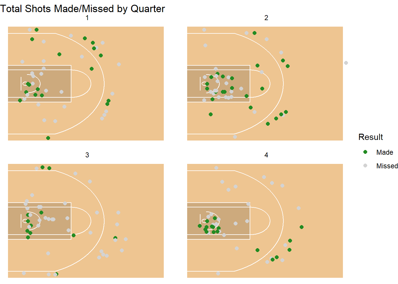
# Save plot for blog
# ggsave("ACBbyfacet.jpg",ACBbyfacet )
# Animate using the new gganimate function transition_states
anim <- allseason +
labs(title = "Game quarter: {closest_state}")+
transition_states(Quarter,wrap =FALSE) +
enter_appear() +
exit_fade(alpha=0)
anim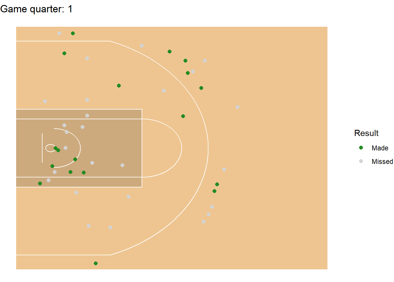
# Save animation for blog
# anim_save("anim.gif",anim)
It does appear from these high level plots and animation that the players shoot closer to the hoop in quarter 4. Is this because they are under time and opposition defense pressure individually or is it part of a team game strategy?
Conclusions
In this post I described how I created an animation of basketball shots data using R.
It was also good to try out the updated version of gganimate and new functions after the listening to the Grammar of animation keynote at useR2018. I had to update from version 0.1.1 to 1.0.0 due to the package revisions and install the gifski R package for the animations to work.
On workflow note, I use blogs as one way to improve the efficiency of my end to end workflow. I try to explore a variety of subject matter with the objective of getting something published within a self imposed deadline. Over and above improving and practing my coding and writing skills, I believe this is also good debugging experience. In this example my initial animations were not as expected, the shot spots were moving around ie persisting between states. I discovered that the group aesthetic was key from rereading the package’s vignettes.
References
- The revisions of gganimate has transitioned to a state of release by Thomas Lin Pedersen.
- This Animating NBA Play by Play using R James blog by P Curley was inspiration for the animation.
- The full court plot court by Ed Küpfer was used as the basis for the half court plot.