- Introduction
- Data Overview
- Load Data
- Data Manipulation
- Data Exploration
- Data Visualisation
- Conclusions
Introduction
The Kaikoura earthquake happened just after midnight on 14 November 2016.
After reading this article Astonishing Nasa photos show Kaikoura land raised by earthquake I thought it would interesting to look at what open data is available to view the land changes from the article.
This analysis has the following objectives:
- Import, manipulate and visualise both vector and raster spatial data
- Use different spatial extents
- Use LiDAR remote sensing open data
- Explore and use different Coordinate Reference System formats including proj.4, EPSG and WKT
- Reproject vector and raster data to different CRS
# Tidyverse metapackage
library(tidyverse)
# Package for reading spatial datasets
library(rgdal)
library(raster)
# Package for manipulating and plotting spatial data
library(sf)
# Package for downloading OSM data
library(osmdata)
# Package for plotting OSM basemap
library(osmplotr)
# Package for interactive maps
library(leaflet)
# Package for raster vis
library(rasterVis)
Data Overview
LiDAR Data
LiDAR or Light Detection and Ranging is an active remote sensing system that can be used to measure vegetation height across wide areas.
LiDAR DEM data from before the earthquakes is available for Kaikoura, Canterbury, New Zealand 2012:
Lidar was captured for Environment Canterbury Regional Council by Aerial Surveys in 2012. Note that this capture was prior to the significant vertical and horizontal displacements from the 2016 Kaikoura earthquakes. The datasets were generated by Aerial Surveys and their subcontractors. The survey area includes the Kaikoura township area and adjacent coastal strips. Data management and distribution is by Land Information New Zealand.
Load Data
Create a Kaikoura Bounding Box
Let’s create a bounding box or bbox which can be described as the spatial extent of the area of Kaikoura we want to initially analyse.
Create a bbox using the getbb function from osmdata R package of Kaikoura town.
# Get longitude and latitude coordinates for a Kaikoura bbox using osmdata package
kaikoura_bbox<- getbb("Kaikoura")
# Take a look at the CRS
crs(kaikoura_bbox)
## [1] NA# Plot the bbox
plot(kaikoura_bbox)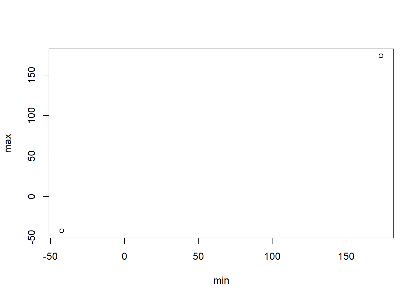
Currently this bbox object has no CRS and it consists of two points? Ideally we would like a polygon shape. Let’s get the bbox as an sf object after following the package examples.
# Get Kaikoura bbox polygon seeting the format to sf
kaikoura_bbox_sf<- osmdata::getbb("Kaikoura", format_out = "sf_polygon")
## No polygonal boundary for Kaikoura# View the kaikoura_bbox_sf
kaikoura_bbox_sf## Simple feature collection with 1 feature and 0 fields
## geometry type: POLYGON
## dimension: XY
## bbox: xmin: 173.6404 ymin: -42.44037 xmax: 173.7204 ymax: -42.36037
## epsg (SRID): 4326
## proj4string: +proj=longlat +datum=WGS84 +no_defs
## geometry
## 1 POLYGON ((173.6404 -42.3603...# We can check the bbox extent of our sf object using st_bbox function
st_bbox(kaikoura_bbox_sf)## xmin ymin xmax ymax
## 173.64036 -42.44037 173.72036 -42.36037# Check the crs of the bbox
st_crs(kaikoura_bbox_sf)## Coordinate Reference System:
## EPSG: 4326
## proj4string: "+proj=longlat +datum=WGS84 +no_defs"# Now plot the bbox sf object using ggplot and geom_sf to check that it is a box/pologon
ggplot(kaikoura_bbox_sf)+
geom_sf()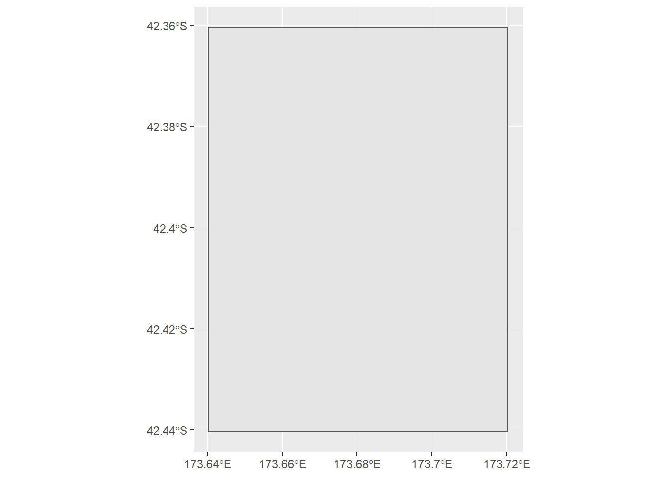
The Coordinate Reference System (CRS) is the WGS84 (EPSG 4326) system:
OpenStreetMap uses the WGS84 spatial reference system used by the Global Positioning System (GPS). It uses geographic coordinates between -180° and 180° longitude and -90° and 90° latitude. So this is the “native” OSM format.
Let’s plot this bbox using leaflet R package to see where it is on a map.
# Map Kaikoura using leaflet and the bbox
kaikoura_bbox_sf %>%
      leaflet() %>%
      addTiles() %>%
      addPolylines()
Longitude and latitude is useful for navigation and locating places on a map but not for data analysis or measurement so we need use a consistent map projection for all our data.
Maps of New Zealand used for data analysis use New Zealand Transverse Mercator / New Zealand Geodetic Datum 2000 (EPSG:2193).
Now we want to project the bbox to EPSG 2193 which is in metres instead of degrees. We will create a Well-known text (WKT) polygon to export to and load in QGIS to visualise the raster data sets within this bbox.
# Change the Epsg of the bbox to EPSG 2193 for NZ using st_transform
kaikoura_bbox_sf_2193<- st_transform(kaikoura_bbox_sf,2193)
# Check the crs of the transformed bbox
st_crs(kaikoura_bbox_sf_2193)
## Coordinate Reference System:
## EPSG: 2193
## proj4string: "+proj=tmerc +lat_0=0 +lon_0=173 +k=0.9996 +x_0=1600000 +y_0=10000000 +ellps=GRS80 +towgs84=0,0,0,0,0,0,0 +units=m +no_defs"# We can check the bbox extent of our reprojected sf object in metres using st_bbox function
st_bbox(kaikoura_bbox_sf_2193)## xmin ymin xmax ymax
## 1652666 5301077 1659321 5310012# Create a WKT from the bbox class using sf package
Kaikoura_WKT <- st_as_text(st_geometry(kaikoura_bbox_sf_2193)) %>%
data.frame()
# Write the WKT to file to be imported into QGIS
# write_csv(Kaikoura_WKT,"kaikoura_wkt.csv")Import the LiDAR Data
Import the LiDAR data in raster or gridded format using the raster R package. We will first inspect one sample tif file as there are a large number of files from the downloaded zip file.
The GeoTIFF format contains a set of embedded or tif tags with metadata about the raster data. We can use the function GDALinfo() from rgdal R package to get information ie metadata about our raster data before we read that data into R. It is ideal to do this before importing your data.
# Preview metadata using GDALinfo from rgdal package
GDALinfo("data/DEM_BT27_2012_1000_4343.tif")
## rows 720
## columns 480
## bands 1
## lower left origin.x 1656160
## lower left origin.y 5303040
## res.x 1
## res.y 1
## ysign -1
## oblique.x 0
## oblique.y 0
## driver GTiff
## projection +proj=tmerc +lat_0=0 +lon_0=173 +k=0.9996 +x_0=1600000
## +y_0=10000000 +ellps=GRS80 +towgs84=0,0,0,0,0,0,0 +units=m
## +no_defs
## file data/DEM_BT27_2012_1000_4343.tif
## apparent band summary:
## GDType hasNoDataValue NoDataValue blockSize1 blockSize2
## 1 Float32 TRUE -9999 256 256
## apparent band statistics:
## Bmin Bmax Bmean Bsd
## 1 2.88 75.63 36.40099 22.00292
## Metadata:
## AREA_OR_POINT=Area# Import raster sample file with raster package
lidar_sample <- raster(x = "data/DEM_BT27_2012_1000_4343.tif")
# Take a look at the class of this object
class(lidar_sample)## [1] "RasterLayer"
## attr(,"package")
## [1] "raster"# Check the CRS of the lidar sample file
crs(lidar_sample)## CRS arguments:
## +proj=tmerc +lat_0=0 +lon_0=173 +k=0.9996 +x_0=1600000
## +y_0=10000000 +ellps=GRS80 +towgs84=0,0,0,0,0,0,0 +units=m
## +no_defsThe file is a “RasterLayer”, a single layer of raster data and the CRS is in proj.4 format with the transverse Mercator projection:
- proj=tmerc
- k=0.9996 Scale factor. Determines scale factor used in the projection.
- x_0=1600000 False easting
- y_0=10000000 False northing
- units=m: the units for the coordinates are in METERS
- ellps=GRS80: the ellipsoid (how the earth’s roundness is calculated) for the data is GRS80
Each LiDAR point has an elevation value, which adds a third dimension to the spatial data.
# Create a list of the file paths of the tif files and select rasters DEM_BT27_2012_1000_434*.tif based on a more detailed area we look for to analyse based on QGIS analysis using glob2rx function https://stackoverflow.com/questions/14360174/list-files-pattern-argument-in-r-extended-regular-expression-use
list_tifs <- list.files(path = "data/", pattern = glob2rx("DEM_BT27_2012_1000_434*.tif"), full.names = TRUE)
# Create a list of raster layers from the list_tifs
raster_list <- map(list_tifs, raster)
# Take a look at the first raster in the list
raster_list[[1]]
## class : RasterLayer
## dimensions : 720, 480, 345600 (nrow, ncol, ncell)
## resolution : 1, 1 (x, y)
## extent : 1655200, 1655680, 5303040, 5303760 (xmin, xmax, ymin, ymax)
## coord. ref. : +proj=tmerc +lat_0=0 +lon_0=173 +k=0.9996 +x_0=1600000 +y_0=10000000 +ellps=GRS80 +towgs84=0,0,0,0,0,0,0 +units=m +no_defs
## data source : C:\Users\Home\Documents\blogdown_source\content\post\data\DEM_BT27_2012_1000_4341.tif
## names : DEM_BT27_2012_1000_4341
## values : -0.75, 3.98 (min, max)Data Manipulation
Now let’s manipulate the data that we have imported. First merge the LiDAR rasters.
# Now use the raster merge function to merge the raster layers of the lidar data
kaikoura_lidar <- do.call(raster::merge, c(raster_list, tolerance = 1))
# Write the merged raster as object for QGIS
# writeRaster(kaikoura_lidar,"kaikoura_lidar.tiff")
Let’s check the extents of the raster sets.
# Check the extent of the lidar raster
extent(kaikoura_lidar)
## class : Extent
## xmin : 1655200
## xmax : 1659520
## ymin : 5303040
## ymax : 5303760Next we will create and visualise an Area of Interest (AOI) from the LiDAR rasters. These capture areas where the seabeds lifted after the Kaikoura earthquake.
# Created AOI from the lidar raster extent
AOI <- as(extent(kaikoura_lidar),'SpatialPolygons')
# Set the CRS to the lidar data proj4string
crs(AOI)@projargs <- crs(kaikoura_lidar)@projargs
# Create a sf object
AOI_sf <- st_as_sf(AOI)
# Set the CRS to EPSG 2193
AOI_sf <- st_transform(AOI_sf,2193)
# Check the crs of the transformed bbox
st_crs(AOI_sf)## Coordinate Reference System:
## No EPSG code
## proj4string: "+proj=tmerc +lat_0=0 +lon_0=173 +k=0.9996 +x_0=1600000 +y_0=10000000 +ellps=GRS80 +towgs84=0,0,0,0,0,0,0 +units=m +no_defs"# We can check the bbox extent of our reprojected sf object is in metres using st_bbox function
st_bbox(AOI_sf)## xmin ymin xmax ymax
## 1655200 5303040 1659520 5303760# Create a WKT from the bbox class using sf package
AOI_WKT <- st_as_text(st_geometry(AOI_sf)) %>%
data.frame()
# Write the WKT to file to be imported into QGIS
# write_csv(AOI_WKT,"AOI_wkt.csv")# Set the EPSG to the native OSM EPSG 4326 https://rstudio.github.io/leaflet/projections.html for purposes of visualising the AOI rather than customing the leafletCRS to EPSG: 2193
AOI_sf_4326 <- st_transform(AOI_sf,4326)
# Map AOI using leaflet
m<- AOI_sf_4326 %>%
leaflet() %>%
addTiles() %>%
addPolylines()
m# Save htmlwidget for blog post
# htmlwidgets::saveWidget(m,"AOI.html")Now convert the merged LiDAR raster to a dataframe.
# Convert the raster data to a dataframe
kaikoura_lidar_df <- as.data.frame(kaikoura_lidar, xy = TRUE)
Data Exploration
Now plot the distribution of elevation values within the area of interest using our LiDAR raster data.
# plot histogram using ggplot
ggplot(kaikoura_lidar_df,aes(layer)) +
      geom_histogram()+
      ggtitle("Distribution of surface elevation values") +
      xlab("Elevation (meters)") +
      ylab("Frequency")
## `stat_bin()` using `bins = 30`. Pick better value with `binwidth`.## Warning: Removed 433655 rows containing non-finite values (stat_bin).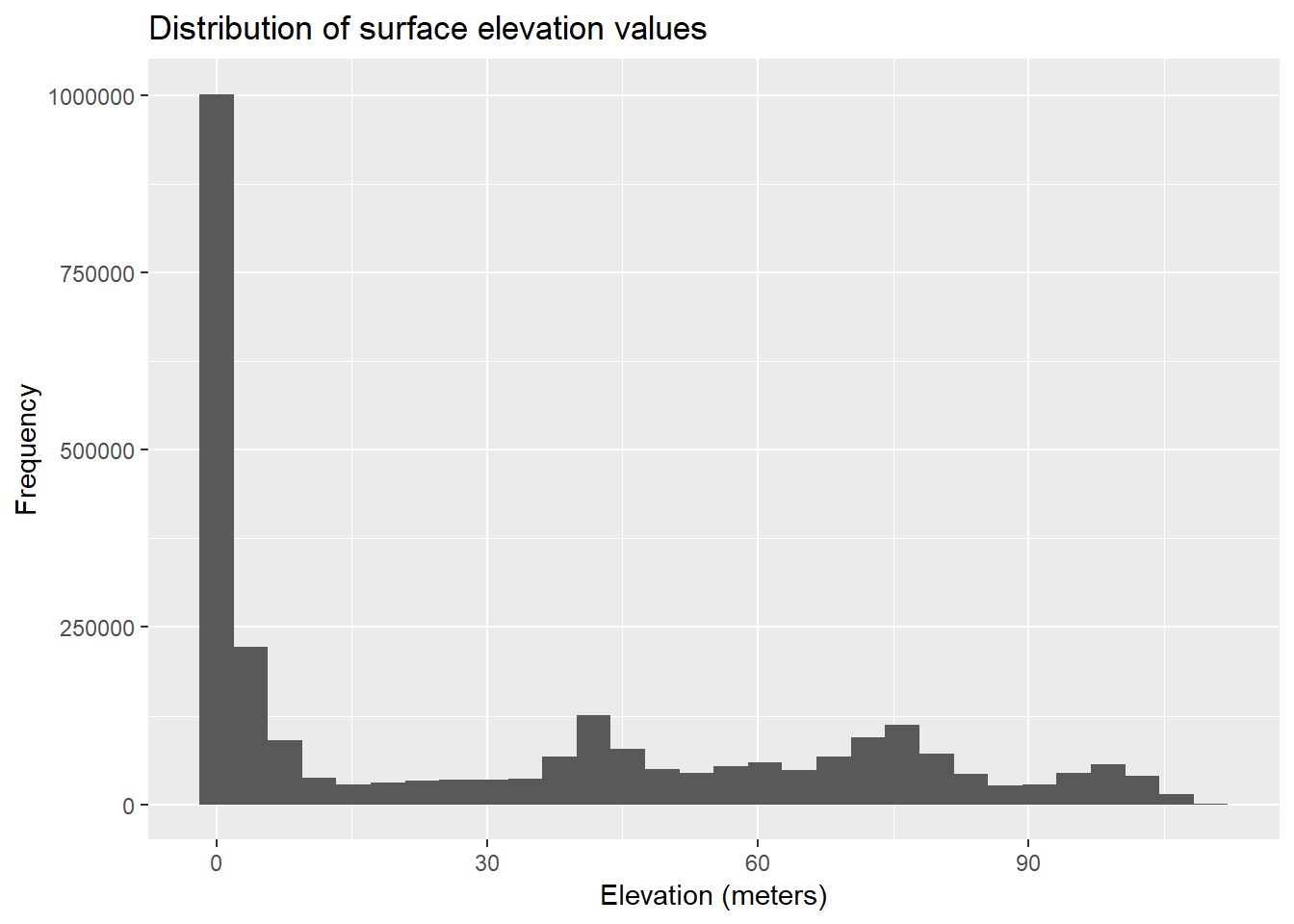
# Find the highest point in the AOI
highest_point <- kaikoura_lidar_df %>%
      top_n(1)
## Selecting by layerhighest_point## x y layer
## 1 1656957 5303102 108.7From this histogram it seems this coastal land has some flat sea level land and steep sections to hilly viewpoints.
We could use LiDAR data from after the earthquake to measure the earth and seabed movements from the elevation differences if this data is made available by LINZ.
Data Visualisation
Let’s visualise the LiDAR raster in our AOI using base plot and levelplot from the rasterVis R package.
# Use base plot to plot the lidar raster with the highest point
plot(kaikoura_lidar,sub="Source: LINZ CC 4.0") + title("Digital Elevation Model (DEM) Data \n Kaikoura, New Zealand \n Before the Earthquake in 2012")
## integer(0)points(highest_point,col="green",pch = 19)
# Plot levelplotusing rasterVis package
levelplot<- levelplot(kaikoura_lidar, layers = 1, margin = list(FUN = 'median'), contour=TRUE)
levelplot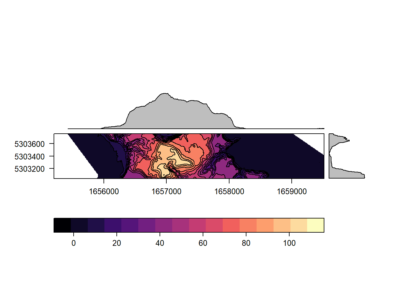
Now let’s view a recent satellite imagery so see what the sea beds look like now.
# Map AOI using leaflet with satellite basemap
m2 <- AOI_sf_4326 %>%
      leaflet() %>%
      addTiles() %>%
      addProviderTiles(providers$Esri.WorldImagery) %>%
      addPolylines()
m2
# htmlwidgets::saveWidget(m2,"SatelliteAfterQuakes.html")We can see the raised sea beds from the earthquake in the leaflet satellite plot.
Conclusions
This has been a great venture into using raster data and different coordinate systems. One of the main challenges with this type of data is that it is very big and so it is useful to know other tools such as QGIS.
Other lessons learnt include:
- Use base plot in R for initial visualisations of raster data as these data may be very large and using ggplot may just crash your PC.
- Select the appropriate CRS up front in the data analysis and then reproject data. However reprojections of raster datasets can also be memory intensive. Using QGIS for on the fly projections are a good way to take a look at the data.
- Most basic plots use the native OSM unprojected CRM system of WGS84. Since leaflet also defaults to this CRS, this would be the familiar starting point for first attempts at geospatial analysis.
- Another way to view DEM’s is with 3D and there is so much more scope for playing with 3D R packages and other tools.