Introduction
The motivations for cycling around town can be for fitness, economic or environmental reasons. However in Auckland the weather and the 53 odd volcanoes could be deterrents to would-be cyclists.
Auckland Transport (AT) publishes daily and monthly bike count data from counters around Auckland now available under CC BY 4.0 license.
Kia ora, us again! We've had this updated now: https://t.co/OXIZvvmS8f Thanks for bringing this to our attention 😀^JN
— Auckland Transport (@AklTransport) December 16, 2018
We will analyse and visualise this data, then fit a model to forecast Auckland bike activity and trends to see if cyclists are braving the weather and taking on the hills.
Load Packages
# Load the tidyverse metapackage
library(tidyverse)
# Load skimr for summary statistics
library(skimr)
# Load the leaflet and htmltools packages for maps
library(leaflet)
library(htmltools)
# Load the sf package for map coordinate manipulations
library(sf)
# Load the lubridate package for time variable manipulations
library(lubridate)
# Load the forecast package for time series
library(forecast)
# Load the cowplot package for side by side ggplots
library(cowplot)
Data
Import data
Use the read_csv functions from the readr R package to import the csv files directly from urls. These function can be used for most csv files, reading and parsing the files to dataframes.
# Import the bikes daily counter dataset for August
url <- "https://at.govt.nz/media/1977986/august2018akldcyclecounterdata.csv"
bikes_daily <- read_csv(url)
## Parsed with column specification:
## cols(
## .default = col_integer(),
## Date = col_character()
## )## See spec(...) for full column specifications.# Import the bikes mounthly counter dataset. Set the counter variables types to numeric
url2 <-"https://at.govt.nz/media/1975708/monthlyakldcyclecountdatanov2010-dec2017.csv"
bikes_monthly <- read_csv(url2,
col_types = cols(.default = col_number(), Month=col_character()))Data Summaries
View the summary statistics with the skimr R package.
# Produce a skim summary excluding the histograms as these do not plot in R markdown currently
skim_with(numeric = list(hist = NULL))
skim_with(
  numeric = list(p0 = NULL, p25 = NULL, p50 = NULL, p75 = NULL, p100 = NULL,sd = NULL,hist = NULL),
  integer = list(p0 = NULL, p25 = NULL, p50 = NULL, p75 = NULL, p100 = NULL,sd = NULL,hist = NULL)
)
skim(bikes_daily)
## Skim summary statistics
## n obs: 32
## n variables: 42
##
## -- Variable type:character ------------------------------------------------------------
## variable missing complete n min max empty n_unique
## Date 1 31 32 14 15 0 31
##
## -- Variable type:integer --------------------------------------------------------------
## variable missing complete n mean
## Beach Road Cyclists 1 31 32 275.9
## Carlton Gore Cycle Counter Cyclists 1 31 32 225.94
## Curran Street Total Cyclists 1 31 32 248.23
## Dominion Road Total Cyclists 1 31 32 295.55
## East Coast Road Cyclists 1 31 32 88.65
## GI TO TAMAKI DR SECTION-1 Cyclists 1 31 32 20.19
## Grafton Bridge Cyclists 1 31 32 550.87
## Grafton Gully Cyclists 1 31 32 347.23
## Grafton Road Cyclists 1 31 32 81.29
## Great North Rd Total Cyclists 1 31 32 226.1
## Great South Rd Total Cyclists 1 31 32 80.71
## HighBrook Cyclists 1 31 32 37.9
## Hopetoun Street Cyclists 1 31 32 159.03
## Karangahape Road Cyclists 1 31 32 456.9
## Lagoon Drive Cyclists 1 31 32 142.13
## Lake Road Total Cyclists 1 31 32 320.29
## Mangere Bridge Cyclists 1 31 32 322.68
## Mangere Safe Routes Cyclists 1 31 32 18.61
## Matakana Cyclists 1 31 32 14.97
## Nelson Street Cyclists 1 31 32 419.9
## Nelson Street Lightpath Cyclists 1 31 32 383.23
## NW Cycleway Kingsland Cyclists 1 31 32 794.23
## NW Cycleway TeAtatu Cyclists 1 31 32 607.55
## Oceanview Rd Waiheke Cyclists 1 31 32 92.32
## Orewa Path Cyclists 1 31 32 240.35
## Ormiston Rd Total Cyclists 1 31 32 48.48
## Pukekohe - Queen St Cyclists 1 31 32 9.06
## Quay St Eco Display Cyclists 1 31 32 828.58
## Quay St Spark Arena Total Cyclists 1 31 32 575.45
## Rankin Ave Cyclists 1 31 32 23.45
## Saint Lukes Rd Total Cyclists 1 31 32 170.94
## SW Shared Path Cyclists 1 31 32 165.26
## Symonds St Total Cyclists 1 31 32 361.77
## Tamaki Drive Total Cyclists 1 31 32 1138.06
## TeAtatu Peninsula Pathway Cyclists 1 31 32 151.55
## TeWero Bridge Bike Counter Cyclists 1 31 32 582.13
## Twin Streams Cyclists 1 31 32 83.65
## Upper Harbour Cyclists 1 31 32 136.03
## Upper Queen Street Cyclists 1 31 32 127.52
## Victoria Street West Total Cyclists 1 31 32 114.94
## Waterview Unitec Counter Cyclists 1 31 32 174.81The bikes_daily dataset has the following variables in wide format:
Date : daily from Wed 1 Aug 2018
Bike counter street location names : 41 locations
It seems like the last row consists of NAs, so we can remove this row in the cleaning step.
# Produce a skim summary excluding the histograms as these do not plot in R markdown currently
skim(bikes_monthly)
## Skim summary statistics
## n obs: 87
## n variables: 42
##
## -- Variable type:character ------------------------------------------------------------
## variable missing complete n min max empty n_unique
## Month 0 87 87 6 11 0 87
##
## -- Variable type:numeric --------------------------------------------------------------
## variable missing complete n mean
## Beach Rd 48 39 87 8537
## Canada St 85 2 87 1067
## Carlton Gore Rd 58 29 87 6008.21
## Curran St 61 26 87 8046.12
## Dominion Rd (near Balmoral Rd) 51 36 87 3391.72
## Dominion Rd (near View Rd) 82 5 87 8959.6
## East Coast Rd 24 63 87 3880.1
## G Sth Road 1 86 87 2684.43
## Glen Innes (Te Ara ki Uta ki Tai) 73 14 87 658.64
## Grafton Bridge 26 61 87 14727.38
## Grafton Gully 48 39 87 9556.64
## Grafton Rd 61 26 87 2291.31
## Gt Nth Rd (citybound only until May 2017) 70 17 87 5030.88
## Highbrook 1 86 87 1162.44
## Hopetoun St 61 26 87 4317
## K Rd 49 38 87 15239
## Lagoon Dr 25 62 87 5166.73
## Lake Road 1 86 87 8714.14
## Mangere Bridge 11 76 87 12440.62
## Mangere Safe Routes 70 17 87 1233.41
## Matakana Bridge 85 2 87 679
## Nelson St cycleway 62 25 87 10846
## Nelson St Lightpath 62 25 87 14633.92
## NW Cycleway \n(Te Atatu) 1 86 87 12861.63
## NW Cycleway (Kingsland) 1 86 87 14751.98
## Oceanview Rd, Waiheke 86 1 87 6086
## Orewa 1 86 87 8587.48
## Ormiston Rd Flat Bush 85 2 87 1194.5
## Pukekohe Queen St 85 2 87 264
## Quay St Spark Arena 61 26 87 32134.92
## Quay St totem 69 18 87 23498.89
## SH20 Dom Rd 25 62 87 3140.39
## St Luke's Rd 80 7 87 5307.29
## Symonds St 49 38 87 11254.61
## Tamaki Dr (EB + WB) 18 69 87 34166.7
## Te Wero Bridge 56 31 87 17058.1
## Twin Streams 1 86 87 3315.06
## Upper Harbour 1 86 87 4345.03
## Upper Queen St 61 26 87 4198.5
## Victoria St West 61 26 87 3927.35
## Waterview SP (Unitec) 82 5 87 4907.4The bikes_monthly dataset has the following variables in wide format:
Date : monthly from Nov-10
Bike counter street location Names : 41 locations
There are missing values represented as NA’s to be considered in data aggregations.
This analysis will assume that the bike counter data is accurate in counting cyclists as we have no visibility of the apparatus or data storage.
Auckland Population Data
Population estimates for regional council, territorial authority (including Auckland local board), area unit, and urban areas is available from DataHub table viewer. In order to download the data, a request needs to be submitted online but the Stats NZ link doesn’t currently work. As an interim workaround, a manual dataframe is created based on the online query results.
# Create Auckland population dataset
population <- data.frame(Date= c("30-June-11","30-June-12","30-June-13","30-June-14","30-June-15",         "30-June-16","30-June-17"), Auckland = c(1459600, 1476500, 1493200, 1526900, 1569900, 1614500, 1657200   ))
Data Cleaning
The bikes_daily and bikes_monthly counter data do not have coordinates available so we will manually create a dataframe with selected points with the longitude and latitude coordinates from a GPS coordinates lookup website.
- Curran_Street
- Quay_Street
- Grafton_Gully
Feedback has been sent to AT to add the longitude and latitude coordinates to their csv files, so that further mapping and joins with other data can be performed another time.
# Create a streets datafarme
streets <- data.frame(street = c("Curran_Street","Quay_Street","Grafton_Gully"),  longitude=c(174.739289,174.773376,174.7678), latitude=c(-36.840521,-36.844713,-36.8623), stringsAsFactors = FALSE)
Now clean the the bikes_daily and bikes_monthly using dplyr and lubridate R packages.
# Convert the character date variable to a date variable using lubridate
bikes_daily$Date <- dmy(bikes_daily$Date)
# Add a new weekday variable using lubridate and dplyr
bikes_daily <- bikes_daily %>%
      mutate(weekday =weekdays(Date)) %>%
      # Remove the last row with NAs in the dataframe using slice using this tip https://stackoverflow.com/questions/38916660/r-delete-last-row-in-dataframe-for-each-group
      slice(-n())

# View the column names by position in bikes_daily to check they are the 3 points we have selected
names(bikes_daily)[4]
## [1] "Curran Street Total Cyclists"names(bikes_daily)[9]## [1] "Grafton Gully Cyclists"names(bikes_daily)[29]## [1] "Quay St Eco Display Cyclists"# Rename the 3 points in bikes_daily to match the streets points
names(bikes_daily)[4] <- streets[1,1]
names(bikes_daily)[9] <- streets[2,1]
names(bikes_daily)[29] <- streets[3,1]
# View the column names by position in bikes_monthly to check they are the 3 points we have selected
names(bikes_monthly)[5]## [1] "Curran St"names(bikes_monthly)[11]## [1] "Grafton Gully"names(bikes_monthly)[32]## [1] "Quay St totem"# Rename the 3 points in bikes_monthly to match the streets points
names(bikes_monthly)[5] <- streets[1,1]
names(bikes_monthly)[11] <- streets[2,1]
names(bikes_monthly)[32] <- streets[3,1]
# Add the row sums ignoring the NAs and remove the first row which has a month as Te Atatu
bikes_monthly <- bikes_monthly %>%
mutate(sumStreets = rowSums(.[2:dim(bikes_monthly)[2]],na.rm = TRUE)) %>%
slice(-1)
# Convert the character date variable to a date variable using lubridate
bikes_monthly$Month <- dmy(paste0("01-", bikes_monthly$Month))
# In order to select the bikes columns as the vector of points in the streets dataframe, we need to provide column names as variables which contain strings. We could use select_ as the standard evaluation counterpart of select. However from the docs select_ has been deprecated in favour of tidy eval. https://timmastny.rbind.io/blog/nse-tidy-eval-dplyr-leadr/#expressions. We use the unquote !! https://adv-r.hadley.nz/quasiquotation.html to tell dplyr to select the variables that match the values in the streets$street vector and combine with the Date and weekday variable in the bikes dataset
bikes_subset <- bikes_daily %>%
select(!!streets$street) %>%
cbind(bikes_daily %>% select(Date,weekday))
# Now convert this dataframe into a tidy dataset using gather, where the Key is the street and the value is the count http://garrettgman.github.io/tidying/
bikes_subset <- bikes_subset %>%
gather(key = "street", value="counts",1:3)
# Now join the streets coordinates and the bikes subset dataframe using dplyr function inner_join
bikes_streets <- streets %>%
inner_join(bikes_subset,by = "street")# Creat a sf object from the streets dataframe with points geometries with crs as 2193 https://epsg.io/2193
bikes_streets_sf <- st_as_sf(bikes_streets,
coords = c("longitude", "latitude"), crs=2193)Visualisations
Bike Counter Locations Daily Data
Let’s visualise the selected bike counter locations using the leaflet R package.
# Create a leaflet map centred at the mean of the streets points
long <- mean(streets$longitude)
lat <- mean(streets$latitude)
m <- leaflet() %>%
      setView(lng = long, lat = lat, zoom = 13) %>%
      addTiles()
m %>%
      addMarkers(data = bikes_streets_sf,
                 popup = ~htmlEscape(street)) %>%
      addProviderTiles(providers$ Stamen.TonerBackground)
Let’s view the daily counts by the 3 counter points with scatter plot and labelled scatterplot, with the regression trend line.
# Plot a facetted plot of the  daily bike counts
ggplot(bikes_streets,aes(Date,counts))+
      geom_point() +
      geom_smooth(method="lm") +
      facet_wrap(~street) +
      theme_bw()+
      ggtitle("Daily Bicycle Counts and Weekdays for Counter Locations")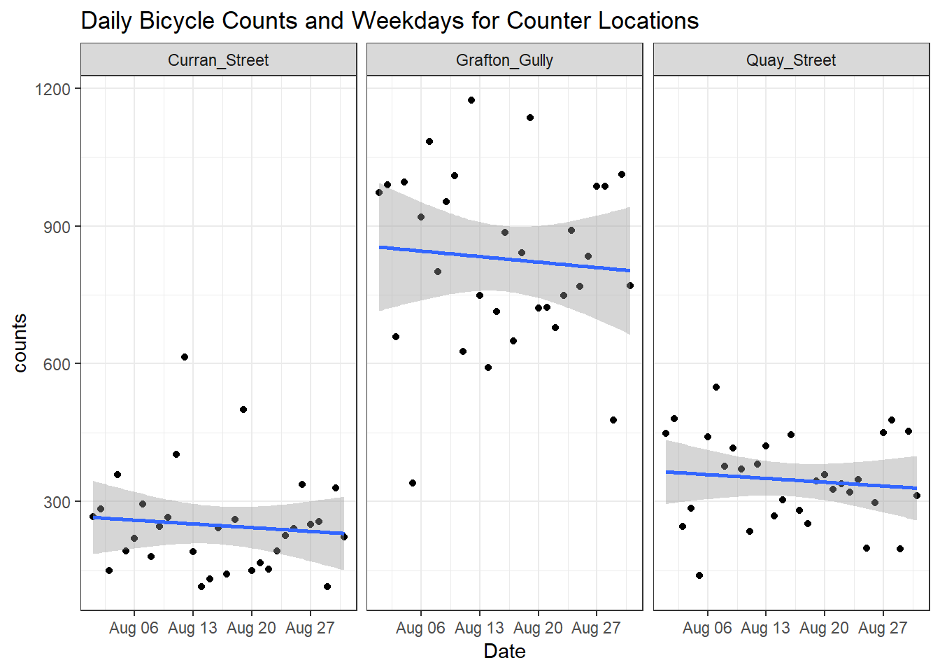
# Plot a facetted plot of the  daily bike counts
ggplot(bikes_streets,aes(Date,counts))+
      geom_point() +
      geom_label(aes(label=weekday)) +
      geom_smooth(method="lm") +
      facet_wrap(~street) +
      theme_bw()+
      ggtitle("Daily Bicycle Counts and Weekdays for Counter Locations")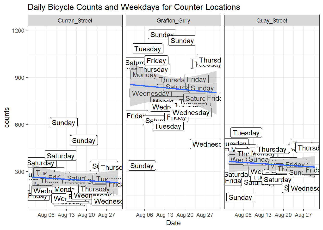
It seems like there is a downward trend for August, perhaps this is related to the winter weather in August?
Next create a ggplot of the total aggregated count by weekday and street.
# Create a gpplot of the total aggregated count by weekday and street
bikes_streets %>%
      group_by(weekday,street) %>%
      summarise(weekday_sum=sum(counts)) %>%
      na.omit() %>%
      # Plot the weekday sum of counts and order the factor levels of the weekday variable but then use forcats fc_rev to reverse the ordering of labels when we add the coord_flip
      ggplot(aes(forcats::fct_rev(factor(weekday, c("Monday", "Tuesday", "Wednesday", "Thursday","Friday", "Saturday","Sunday"))) , weekday_sum, fill=street))  +
      geom_col(position="dodge") +
      scale_fill_viridis_d()  +
      xlab("Weekday")+
      ylab("Sum of Weekday Counts") +
      coord_flip()  +
      theme_bw() +
      ggtitle("Total Aggregated Bicyle Count by Weekday and Street")+
      labs(caption = "Source: AT https://at.govt.nz/cycling-walking/research-monitoring/")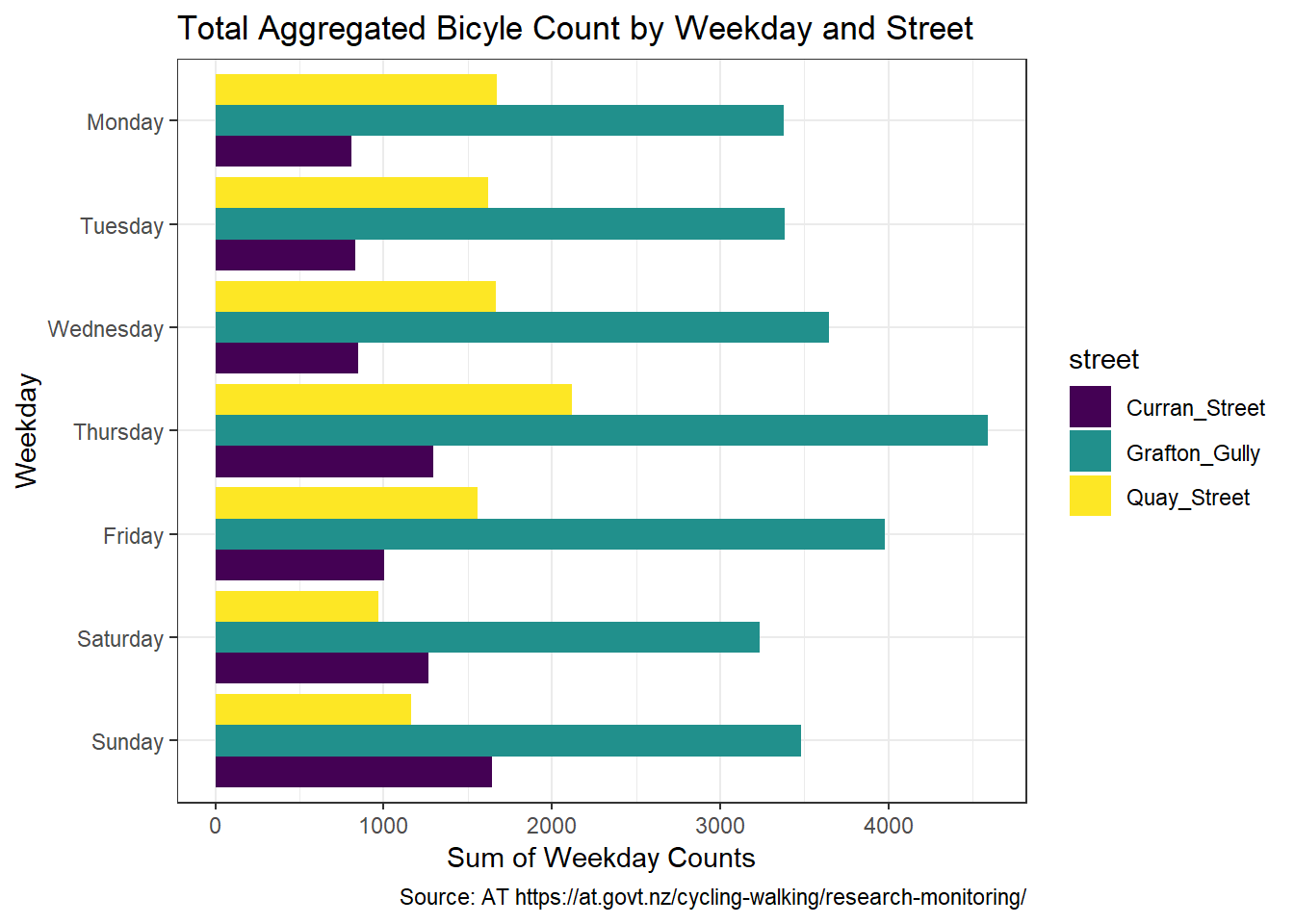
Weekdays notably Thursday appears to be the most popular day in Grafton Gully and Quay Street, but Sunday appears the most popular day for cycling in Curran Street.
Bike Counter Locations Monthly Aggregated Data
Now lets turn to the monthly bike count dataset bike_monthly and look at this as a time series.
First we will use the base decompose function to break the time series into its components.
# Create a time series object bikes_monthly_ts
bikes_monthly_ts <- ts(bikes_monthly$sumStreets, start=c(2010,11), frequency=12)
decomp <- decompose(bikes_monthly_ts)
# Plot the decomposed time series
autoplot(decomp)
From the decomposed components it appears there is a repetitive seasonality pattern dipping in winter months and an overall upwards trend.
Compare Aggregated Bike Data with another Dataset
Now extract and plot the trend line against another dataset. Here we will use the Auckland population data over a similar time period.
# Plot the Auckland population
population$Date <- dmy(population$Date)
pop_ts <- ts(population$Auckland, start=c(2011), frequency=1)

bike_trend <- decomp$trend
# Plot the Auckland bicycle growth
bike_plot <- autoplot(bike_trend,na.rm=TRUE) +
      ylab("Bicycle Counts") +
      xlab("Date")+
      scale_y_continuous(labels = scales::comma)+
      ggtitle("Auckland Estimated Bicyle Counts") +
      theme_bw() +
      labs(caption = "Source: AT https://at.govt.nz/cycling-walking/research-monitoring/")
# Plot the Auckland population growth
pop_plot <- autoplot(pop_ts)+xlab("Date") +
      ylab("Population number")+
      scale_y_continuous(labels = scales::comma)+
      ggtitle("Auckland Estimated Population") +
      theme_bw()+
      labs(caption = "Source: NZ Stats http://nzdotstat.stats.govt.nz/")
# Plot side by side plots with cowplot packagefor comparison instead of using 2 y-axis
plot_grid(bike_plot,pop_plot, labels = "AUTO")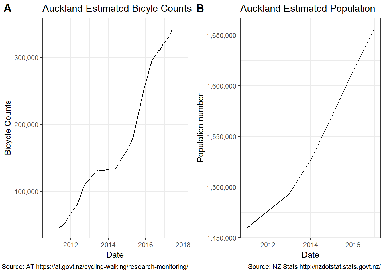
# save_plot("cowplot.png", p, ncol = 2)The cycling trend in A looks remarkably similar to Auckland population growth in B?!? It seems like increasing population is cycling regardless of the hilly roads.
Forecast Bike Numbers
Finally create an arima model using the auto.arima function from the forecast R package to see what the growth in cycling could look like.
# Fit an arima model using auto.arima function
fit <- bikes_monthly_ts %>%
      auto.arima(seasonal=TRUE)
# Produce a summary of the fitted model
summary(fit)
## Series: .
## ARIMA(0,1,1)(2,1,0)[12]
##
## Coefficients:
## ma1 sar1 sar2
## -0.1933 -0.6515 -0.2840
## s.e. 0.1198 0.1203 0.1369
##
## sigma^2 estimated as 365080369: log likelihood=-824.49
## AIC=1656.97 AICc=1657.56 BIC=1666.13
##
## Training set error measures:
## ME RMSE MAE MPE MAPE MASE
## Training set 1445.464 17238.28 12216.95 0.2184844 6.939697 0.2421102
## ACF1
## Training set -0.002190182# Check ACF and PACF plots for model residuals
tsdisplay(residuals(fit), lag.max=45, main='(0,1,1) Model Residuals')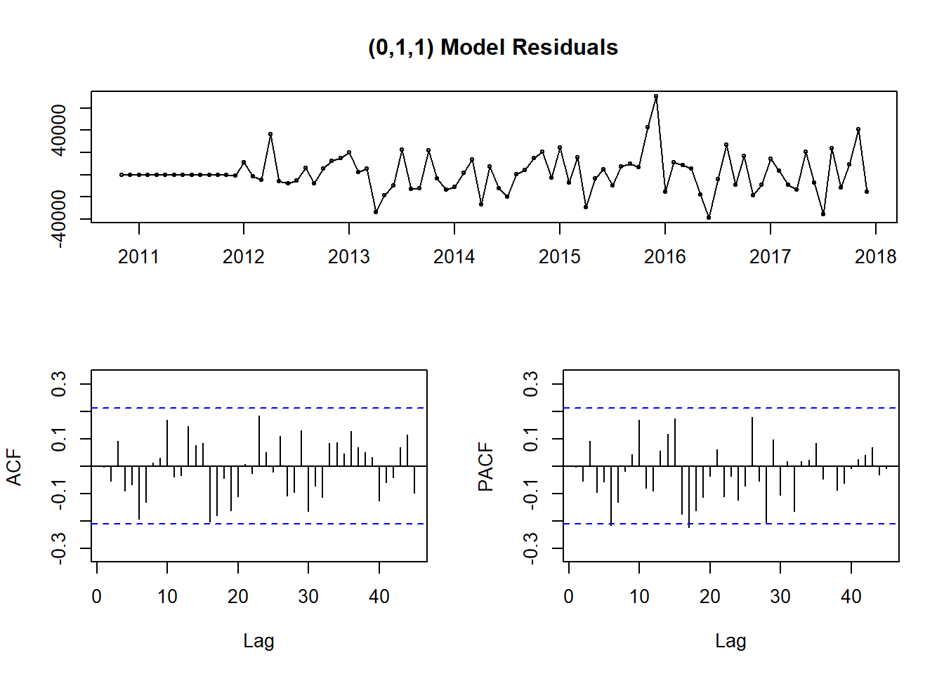
# Plot the forecast using the autoplot function
fit %>%
      forecast() %>%
      autoplot() +
      ylab("Bicycle counts") +
      xlab("Date") +
      scale_y_continuous(labels = scales::comma) +
      scale_x_continuous(labels = scales::number) +
      theme_bw()
## Scale for 'x' is already present. Adding another scale for 'x', which
## will replace the existing scale.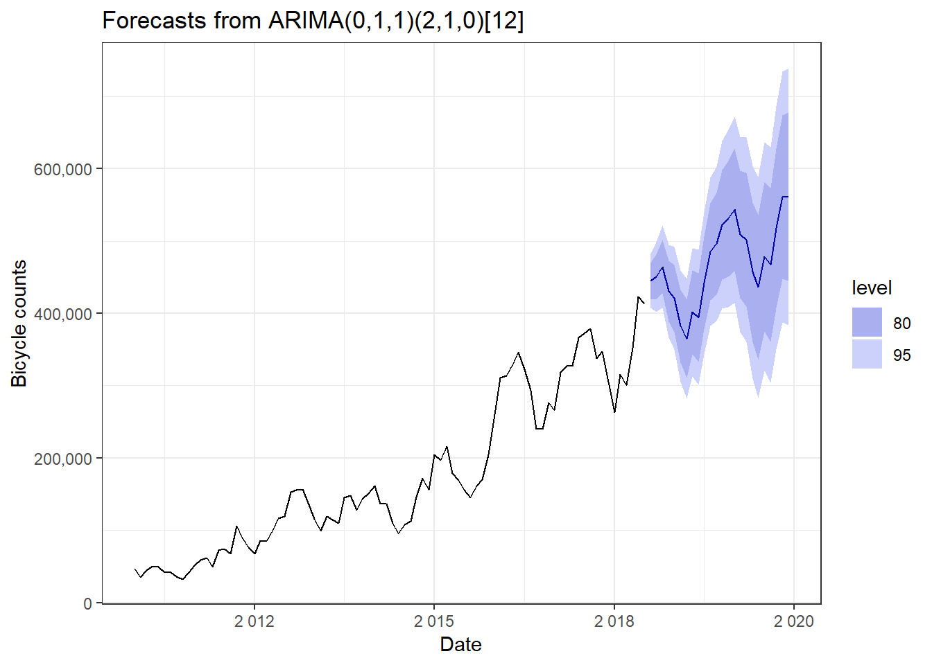
This model is a seasonal Arima model. The moving average model has p=0 autoregressive terms, d=1 , q=1 moving average terms, where d=1 ie differencing of order 1. The seasonal part of the model has P=2 seasonal autoregressive (SAR) terms, D=1 number of seasonal differences, Q=0 seasonal moving average (SMA) terms.
Conclusions
The bike count data is interesting data to look at, especially the time series components and forecast. Once the coordinates are available in the AT datasets, further geospatial analysis can be performed through delving into the sf package and using other data.
The data cleaning here used new functions and packages including lubridate and cowplot and operators including the unquote !! . It has also been good to start reading up on tidy eval.