Introduction
Recently one of the problems I was trying to solve required matrix algebra.

This falls under the umbrella of need to know R basics so I realised I needed a way to track and refresh my R skills, recognise gaps and ultimately create a reference cheat-sheet.
Learning R is a bit of a journey over time so here goes Part 1 of an interactive visualisation project using tidyverse and ggplot compatible1 packages.
# install.packages("tidyverse")
library(tidyverse)
library(ggiraph)
# devtools::install_github("ricardo-bion/ggradar",
#                          dependencies=TRUE)
library(ggradar)
# install.packages("ggiraphExtra")
library(ggiraphExtra)
Data
One of the things every Intro to R course book or course does is provides you with data. However some real life projects need you to create the data, and all projects require you to have some level of understanding of the data so I would argue that when possible create or architect the data yourself.
Also for me, learning works best when the data is personal and relevant. In this project I’ll create dataframes with a self assessment of my own R skills, levels of experience and perceived complexity, tips and dates. I will start with a scale of 1-6 for the numeric data, as it is even.
# Create dataframes
setupR <- data.frame(skill=c("Install RStudio", "Install R","Install R packages","Load Packages", "Update RStudio","Update R", "Update R packages","Basic debugging","Browser debugging"),
                     experience=c(6,6,6,6,6,3,6,5,1),
                     complexity=c(1,1,1,1,1,1,2,1,3),
                     tip=c("","","CRAN install.packages(), GitHub devtools, Jan-19 remotes ","","Nov-18 RStudio packages tab", "","", "Apr-17 Misspelling and punctuation",""),
                     date=c("Apr-17", "Apr-17", "Apr-17", "Apr-17", "Apr-17", "Apr-17", "Nov-18", "Apr-17", ""),
                     stringsAsFactors = FALSE)

objectsR <- data.frame(skill=c("Object assignment","Classes", "Scaler","Vectors","Factors","Matrices", "Arrays", "Dataframes", "Lists","Environments","Tibbles"),
                       experience=c(4,5,5,5,3,5,4,4,3,3,3),
                       complexity=c(3,1,1,1,1,1,1,1,3,3,3),
                       tip=c( "","lubridate for dates", "","c(), a:b, seq(), rep()","forcats", "Feb-19 Use for dataframe manipulation","","data.frame(name = c(),... )","","",""),
                       date=c("Apr-17","Apr-17","Apr-17", "Apr-17", "Apr-17", "Apr-17", "Apr-17", "Apr-17", "Apr-17","Sep-17","Jan-18"),
                       stringsAsFactors = FALSE)

functionsR <- data.frame(skill=c("Create a function", "Vector functions"),
                        experience=c(5,4),
                        complexity=c(1,1),
                        tip=c("function (x) { }","sum(), mean(), sd(), summary(), length(), unique(), table()"),
                        date=c("Apr-17","Apr-17"),
                        stringsAsFactors = FALSE)

importR <- data.frame(skill=c( "txt", "csv", "Excel"),
                      experience=c(5,5,5),
                      complexity=c(2,2,2),
                      tip=c("read.table()" ,"readxl read_csv()","readxl read_xls"),
                      date=c("Apr-17","Jun-17","Jun-17"),
                      stringsAsFactors = FALSE)

exportR <- data.frame(skill=c( "txt", "csv", "Excel"),
                      experience=c(5,5,5),
                      complexity=c(2,2,2),
                      tip=c("write.table()" ,"readxl write_csv()","readxl write_xls"),
                      date=c("Apr-17","Jun-17","Jun-17"),
                      stringsAsFactors = FALSE)

datamungingR <- data.frame(skill=c("Numerical Indexing", "Logical Indexing","Subset","Sorting","Combine","Summarise","Recoding","Reshape","Regex"),
                           experience=c(5,5,3,5,4,4,3,2,2),
                           complexity=c(2,2,2,2,2,3,3,5,5),
                           tip=c("[row,column], [[list]]","operators, & (and), | (or), %in%, is.na(), which()","dplyr select()","order(decreasing = TRUE)","merge(x,y,by=,all=)","aggregate(), dplyr group_by() summarise(n=n())","","tidyr gather() spread()","stringr"),
                           date=c("Apr-17", "Apr-17","Apr-17", "Apr-17", "Apr-17","Apr-17","Jun-17","Jun-17","Jun-17"),
                           stringsAsFactors = FALSE)

vizR <- data.frame(skill=c( "Base plots", "ggplot syntax","ggplot2 themes", "Interactive"),
                   experience=c(1,3,3,3),
                   complexity=c(1,1,3,5),
                   tip=c("","ggplot2","theme_*, Own theme gist", "ggiraph"),
                   date=c("Apr-17","Apr-17","Jun-17","Feb-17"),
                   stringsAsFactors = FALSE)
Take a look at the structure of the first data frame setupR using glimpse from the tibble.
# Summary of setupR dataframe
glimpse(setupR)
## Observations: 9
## Variables: 5
## $ skill <chr> "Install RStudio", "Install R", "Install R packages...
## $ experience <dbl> 6, 6, 6, 6, 6, 3, 6, 5, 1
## $ complexity <dbl> 1, 1, 1, 1, 1, 1, 2, 1, 3
## $ tip <chr> "", "", "CRAN install.packages(), GitHub devtools, ...
## $ date <chr> "Apr-17", "Apr-17", "Apr-17", "Apr-17", "Apr-17", "...This data should be useful for visualisations as the variables have multiple classes. The numeric experience and complexity variables can be used for sizes and coordinates. The date variable can be used to view progress over time (once converted to a date format), and the character skill and tip variables for categories or labels.
With these dataframes as baseline, in order to add new skills create a function to do this, instead of manually updating the dataframes.
# Use readline function to create a prompt to store values in scaler variables, then combine with a vector which can be appended to the dataframe
addskill <- function(df) {
      newname <- readline(prompt="Enter skill name: ")
      newexperience <- readline(prompt="Enter experience (1-5): ")
      newcomplexity <- readline(prompt="Enter experience (1-5): ")
      newtip <- readline(prompt="Enter tip: ")
      newdate <- readline(prompt="Enter date (MMM-YY): ")

      # Create a vector
      newskill <- c(skill=newname,
                    experience=newexperience,
                    complexity=newcomplexity,
                    tip=newtip,
                    date=newdate)
      newskill <- as.data.frame(newskill) %>%
            t()

      rbind(df,newskill)
}
# Use the addskill function
# functionsR <- addskill(functionsR)
# functionsR$experience <- as.numeric(functionsR$experience)
If the datasets have been updated we may need to save them to a file (or database).
# Use write.csv to save dataframes to a flat file
# write_csv(setupR,"setupR.csv")
# write_csv(importR,"importR.csv")
# write_csv(functionsR,"functionsR.csv")
# write_csv(objectsR,"objectsR.csv")
# write_csv(datamungingR,"datamungingR.csv")
# write_csv(vizR,"vizR.csv")
Exploratory Data Analysis
Let’s take a look at some different types of viz of the data.
Barchart
Use ggiraph1 to create an interactive barchart of the setupR dataframe. Use interactive labels to show the tips.
# Create a ggplot object firstg for the setupR dataframe
firstg <- ggplot(data=setupR,
                 # Set the experience as the bar category but keep the ordering as in the dataframe
                 aes(factor(skill, level=skill, ordered=FALSE), experience, fill=experience)) +
      coord_flip()+
      # Use viridis colour palette with plasma as this has a range from blue to yelllow and clearly distinguishes the categories
      scale_fill_viridis_c(option="plasma")+
      ggtitle("R Setup - Self-Assessment of Experience  (1-6)") +
      xlab("")+
      ylab("Experience level") +
      theme_minimal()
# Use ggiraph function to plot an interactive bar chart with the tips as tooltips
ggiraph(code = print(firstg +
                           geom_bar_interactive(aes(tooltip = paste0("Tip: ",tip)),
                                                   show.legend = FALSE,
                                                   size=3,
                                                   stat="identity") ),
        hover_css = "cursor:pointer;font:arial;")
A bar chart may be a good choice for one dataframe but it doesn’t have the flexibility for more groupings or time other than perhaps using facets.
Radar chart
Use ggiraphextra to plot a radar chart. To manipulate the data into the format required as input, use the tidyr R package.
# Use tidyr R package gather and spread to manipulate the data
groupdata <- setupR %>%
   gather(key = group, value = value, 2:ncol(setupR)) %>%
   spread(key = names(setupR)[1], value = "value") %>%
      # Extract one feature of the skillset, the experience, to plot the radar line
      filter(group=="experience") %>%
      # Convert to numeric using dplyr mutate_at
      mutate_at(vars(-group) ,as.numeric)%>%
      # Rescale using dplyr mutate_at
      mutate_at(vars(-group) ,funs(./6))
## Warning: funs() is soft deprecated as of dplyr 0.8.0
## please use list() instead
##
## # Before:
## funs(name = f(.)
##
## # After:
## list(name = ~f(.))
## This warning is displayed once per session.# Now plot radar chart
radar <- ggRadar(data=groupdata,
#https://stackoverflow.com/questions/43644799/r-ggradar-differences-in-behavior-with-interactive-turned-on-or-off
interactive=FALSE,
# Data has been rescaled already in tidying
rescale=FALSE,
colour="blue") +
ggtitle("R Setup - Self-Assessment of Experience (%)") +
# Use ggplot theme_bw to remove greys
theme_bw()+
# Wrap the label text to fit plot area
scale_x_discrete(labels = function(x) str_wrap(x, width = 10)) +
# Make x axis labels smaller to fit area and blank out y axis as the circles are intuitive enough
theme(axis.text.x = element_text(size = 6),
axis.text.y=element_blank(),
axis.ticks.y = element_blank())+
# Remove black panale border
theme(panel.border = element_rect(colour = "white"))
ggiraph(code = print(radar))Radar charts are popoular to chart experience and skills levels. However there are at least 7 datasets grouping different types of skills. Even at 7 overlayed groups, a radar chart may be too complex for this project.
Line roadmap
Now let’s look at line roadmap.
# Create a line road plot function
plotroad <- function(df,colourplot,xstart) {
      # Unit test steps start
      # rm(df)
      # rm(dftoplot)
      # df <- setupR
      # colourplot="blue"
      # xstart<- 4
      # Unit test steps end
      n_road <- dim(df)[1]
      x <- as.numeric(seq(xstart,n_road+xstart-1))
      y <- df$complexity
      dftoplot <- cbind(df,x,y)
      thetitle <- deparse(substitute(df))
      ggplot(data=dftoplot,aes(x,y))+
            ggrepel::geom_text_repel(mapping=aes(label=skill,angle=90),
                                     colour=colourplot,
                                     fontface='bold',
                                     nudge_y = 2,
                                     segment.color = 'grey50')+
            geom_line(data= dftoplot,aes(x,y),
                     # colour=colourplot,
                     size=2,
                      arrow=arrow(type="closed")) +
            geom_point_interactive(aes(x, y, size=experience,
                                       tooltip=paste0("Tip: ",tip)),
                                   colour=colourplot,
                                   #shape=1, Possibly change the shape later
                                   show.legend = TRUE)+
            scale_size_continuous(range = c(1,10))+
            # Add the dataframe name as the title

            ggtitle(paste0("Learning roadmap of ",thetitle))+
            # Set theme for ggplot
            scale_x_discrete()+
            scale_y_discrete()+
            theme_void() +
            theme(plot.title= element_text(family='',
                             face='bold',
                             colour=colourplot,
                             size=15))+
            ylim(c(0,max(y)+3))
}
# View the first ggplot object to  check colour scheme & layout
(g1 <- plotroad(setupR,"blue", 1))
## Scale for 'y' is already present. Adding another scale for 'y', which
## will replace the existing scale.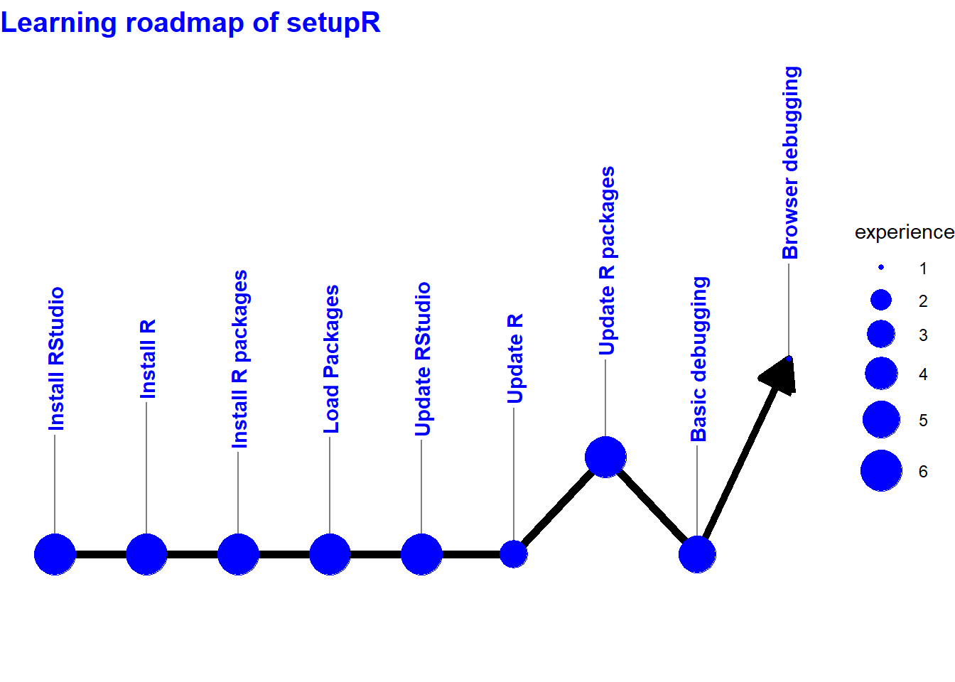
# Use ggiraph to plot an interactive bar chart with the tips as tooltips, let's first create the rest of the ggplot objects for each of the other roads
g2 <- plotroad(objectsR,"red",4)
## Scale for 'y' is already present. Adding another scale for 'y', which
## will replace the existing scale.g3 <- plotroad(importR,"hotpink",4)## Scale for 'y' is already present. Adding another scale for 'y', which
## will replace the existing scale.g4 <- plotroad(functionsR,"darkgreen",2)## Scale for 'y' is already present. Adding another scale for 'y', which
## will replace the existing scale.g5 <- plotroad(datamungingR,"lightblue",10)## Scale for 'y' is already present. Adding another scale for 'y', which
## will replace the existing scale.g6 <- plotroad(vizR,"green",12)## Scale for 'y' is already present. Adding another scale for 'y', which
## will replace the existing scale.# Create an interactive ggplot object
ggiraph(code = print(g1),tooltip_extra_css = "background-color:gray;color:white;font-style:italic;padding:10px;border-radius:5px;fill:white;r:10pt;")First Roadmap
Based on the plots above, I am currently thinking of road map layout, starting at the bottom left and progressing upwards to reflect progression with the tooltips as quick tips. Lines can also be joined or spliced together, whereas bar shapes have limited malleability. Perhaps date becomes a facet to show progress over time? and geospatial concepts can be used to create the roadmap?
Now let’s combine lines into a single plot with gridExtra R package.
# Try out  gridExtra to layout ggplot objects
ggiraph(code = print(gridExtra::grid.arrange(g1,g2,g3,g4,g5,g6, nrow = 6)),tooltip_extra_css = "background-color:gray;color:white;font-style:italic;padding:10px;border-radius:5px;fill:white;r:10pt;")
## TableGrob (6 x 1) "arrange": 6 grobs
## z cells name grob
## 1 1 (1-1,1-1) arrange gtable[layout]
## 2 2 (2-2,1-1) arrange gtable[layout]
## 3 3 (3-3,1-1) arrange gtable[layout]
## 4 4 (4-4,1-1) arrange gtable[layout]
## 5 5 (5-5,1-1) arrange gtable[layout]
## 6 6 (6-6,1-1) arrange gtable[layout]This output is quite busy and not currently malleable. It seems as though the ggplot objects can be plotted side by side, but what about layering and joining the ggplot objects to show the journey?
Conclusions
I have created some data for this project and done some initial data analysis. Through this process, I also reviewed and refreshed some of the fundamentals of the R language and practised some “data architecture”.
Based on the exploratory start to this project, the data appears is usable with the different classes and can be manipulated depending on the requirements of a vis function. The next step is to think more about the interactive roadmap using the fundamentals of data visualisation, see Part 2 for the follow up post.
References
- I really enjoyed reviewing this fun YaRrr! The Pirates Guide to R book as an R refresher and for the data creation.
- A metro line style data scientist roadmap as inspiration for the layout.
1 The reason for this compatibility is to focus on and use a single syntax in this roadmap. The tidyverse is based on tidy data principles and ggplot on the grammar of graphics. The final output for this project could then become a framework for separate learning roadmaps for package wrappers for libraries with different syntax (such as plotly) or different languages (such as Python or D3).